
1.11: Homework problems for Chapter 1
- Page ID
- 21149

\( \newcommand{\vecs}[1]{\overset { \scriptstyle \rightharpoonup} {\mathbf{#1}} } \)
\( \newcommand{\vecd}[1]{\overset{-\!-\!\rightharpoonup}{\vphantom{a}\smash {#1}}} \)
\( \newcommand{\id}{\mathrm{id}}\) \( \newcommand{\Span}{\mathrm{span}}\)
( \newcommand{\kernel}{\mathrm{null}\,}\) \( \newcommand{\range}{\mathrm{range}\,}\)
\( \newcommand{\RealPart}{\mathrm{Re}}\) \( \newcommand{\ImaginaryPart}{\mathrm{Im}}\)
\( \newcommand{\Argument}{\mathrm{Arg}}\) \( \newcommand{\norm}[1]{\| #1 \|}\)
\( \newcommand{\inner}[2]{\langle #1, #2 \rangle}\)
\( \newcommand{\Span}{\mathrm{span}}\)
\( \newcommand{\id}{\mathrm{id}}\)
\( \newcommand{\Span}{\mathrm{span}}\)
\( \newcommand{\kernel}{\mathrm{null}\,}\)
\( \newcommand{\range}{\mathrm{range}\,}\)
\( \newcommand{\RealPart}{\mathrm{Re}}\)
\( \newcommand{\ImaginaryPart}{\mathrm{Im}}\)
\( \newcommand{\Argument}{\mathrm{Arg}}\)
\( \newcommand{\norm}[1]{\| #1 \|}\)
\( \newcommand{\inner}[2]{\langle #1, #2 \rangle}\)
\( \newcommand{\Span}{\mathrm{span}}\) \( \newcommand{\AA}{\unicode[.8,0]{x212B}}\)
\( \newcommand{\vectorA}[1]{\vec{#1}} % arrow\)
\( \newcommand{\vectorAt}[1]{\vec{\text{#1}}} % arrow\)
\( \newcommand{\vectorB}[1]{\overset { \scriptstyle \rightharpoonup} {\mathbf{#1}} } \)
\( \newcommand{\vectorC}[1]{\textbf{#1}} \)
\( \newcommand{\vectorD}[1]{\overrightarrow{#1}} \)
\( \newcommand{\vectorDt}[1]{\overrightarrow{\text{#1}}} \)
\( \newcommand{\vectE}[1]{\overset{-\!-\!\rightharpoonup}{\vphantom{a}\smash{\mathbf {#1}}}} \)
\( \newcommand{\vecs}[1]{\overset { \scriptstyle \rightharpoonup} {\mathbf{#1}} } \)
\( \newcommand{\vecd}[1]{\overset{-\!-\!\rightharpoonup}{\vphantom{a}\smash {#1}}} \)
\(\newcommand{\avec}{\mathbf a}\) \(\newcommand{\bvec}{\mathbf b}\) \(\newcommand{\cvec}{\mathbf c}\) \(\newcommand{\dvec}{\mathbf d}\) \(\newcommand{\dtil}{\widetilde{\mathbf d}}\) \(\newcommand{\evec}{\mathbf e}\) \(\newcommand{\fvec}{\mathbf f}\) \(\newcommand{\nvec}{\mathbf n}\) \(\newcommand{\pvec}{\mathbf p}\) \(\newcommand{\qvec}{\mathbf q}\) \(\newcommand{\svec}{\mathbf s}\) \(\newcommand{\tvec}{\mathbf t}\) \(\newcommand{\uvec}{\mathbf u}\) \(\newcommand{\vvec}{\mathbf v}\) \(\newcommand{\wvec}{\mathbf w}\) \(\newcommand{\xvec}{\mathbf x}\) \(\newcommand{\yvec}{\mathbf y}\) \(\newcommand{\zvec}{\mathbf z}\) \(\newcommand{\rvec}{\mathbf r}\) \(\newcommand{\mvec}{\mathbf m}\) \(\newcommand{\zerovec}{\mathbf 0}\) \(\newcommand{\onevec}{\mathbf 1}\) \(\newcommand{\real}{\mathbb R}\) \(\newcommand{\twovec}[2]{\left[\begin{array}{r}#1 \\ #2 \end{array}\right]}\) \(\newcommand{\ctwovec}[2]{\left[\begin{array}{c}#1 \\ #2 \end{array}\right]}\) \(\newcommand{\threevec}[3]{\left[\begin{array}{r}#1 \\ #2 \\ #3 \end{array}\right]}\) \(\newcommand{\cthreevec}[3]{\left[\begin{array}{c}#1 \\ #2 \\ #3 \end{array}\right]}\) \(\newcommand{\fourvec}[4]{\left[\begin{array}{r}#1 \\ #2 \\ #3 \\ #4 \end{array}\right]}\) \(\newcommand{\cfourvec}[4]{\left[\begin{array}{c}#1 \\ #2 \\ #3 \\ #4 \end{array}\right]}\) \(\newcommand{\fivevec}[5]{\left[\begin{array}{r}#1 \\ #2 \\ #3 \\ #4 \\ #5 \\ \end{array}\right]}\) \(\newcommand{\cfivevec}[5]{\left[\begin{array}{c}#1 \\ #2 \\ #3 \\ #4 \\ #5 \\ \end{array}\right]}\) \(\newcommand{\mattwo}[4]{\left[\begin{array}{rr}#1 \amp #2 \\ #3 \amp #4 \\ \end{array}\right]}\) \(\newcommand{\laspan}[1]{\text{Span}\{#1\}}\) \(\newcommand{\bcal}{\cal B}\) \(\newcommand{\ccal}{\cal C}\) \(\newcommand{\scal}{\cal S}\) \(\newcommand{\wcal}{\cal W}\) \(\newcommand{\ecal}{\cal E}\) \(\newcommand{\coords}[2]{\left\{#1\right\}_{#2}}\) \(\newcommand{\gray}[1]{\color{gray}{#1}}\) \(\newcommand{\lgray}[1]{\color{lightgray}{#1}}\) \(\newcommand{\rank}{\operatorname{rank}}\) \(\newcommand{\row}{\text{Row}}\) \(\newcommand{\col}{\text{Col}}\) \(\renewcommand{\row}{\text{Row}}\) \(\newcommand{\nul}{\text{Nul}}\) \(\newcommand{\var}{\text{Var}}\) \(\newcommand{\corr}{\text{corr}}\) \(\newcommand{\len}[1]{\left|#1\right|}\) \(\newcommand{\bbar}{\overline{\bvec}}\) \(\newcommand{\bhat}{\widehat{\bvec}}\) \(\newcommand{\bperp}{\bvec^\perp}\) \(\newcommand{\xhat}{\widehat{\xvec}}\) \(\newcommand{\vhat}{\widehat{\vvec}}\) \(\newcommand{\uhat}{\widehat{\uvec}}\) \(\newcommand{\what}{\widehat{\wvec}}\) \(\newcommand{\Sighat}{\widehat{\Sigma}}\) \(\newcommand{\lt}{<}\) \(\newcommand{\gt}{>}\) \(\newcommand{\amp}{&}\) \(\definecolor{fillinmathshade}{gray}{0.9}\)- Dynaman.
- Super hero Dynaman is cruising along at 126 km/hr when the Dynamobile suddenly encounters wet pavement and begins hydroplaning. Naturally, Dynamobile is headed straight for a thick, solid steel barrier and will crash if it cannot stop. Also naturally, Dynamobile is equipped not only with conventional brakes (useless against hydroplaning) but also with jet reverse thrusters that can provide emergency braking in the form of a half-sine pulse. Dynaman hits the panic button, which activates all sensors and the onboard computer. The sensors instantly detect initial velocity \(v_0\) = 35.0 m/s, Dynamobile total mass \(m\) = 1 500 kg, and hydroplaning viscous damping constant \(c\) = 7.70 N-s/m. The computer calculates that a possible disaster-avoidance action is to deploy the maximum available braking thrust amplitude of \(F\) = −7 200 N (−7.2 kN) in a half-sine pulse extending over 10.0 s [ \(f_x(t)\) = \(F\sin(0.100\pi t\) for 0 \(\leq\) \(t\) \(\leq\) 10.0 s]. Your task is to demonstrate the effectiveness of this braking thrust by making a MATLAB graph that shows the velocity of Dynamobile over 15 seconds (the 10-s braking period plus another 5 seconds of coasting). Be sure to use good engineering graphical practice: provide grids, a title, appropriate labels, and high point density. Submit your MATLAB script as well as your graph.
- Consider the same scenario as in part (1.1.1), but with the following different data: \(v_0\) = 40.0 m/s, \(m\) = 1 700 kg, \(c\) = 130 N-s/m, with braking force amplitude \(F\) = −30 000 N (−30.0 kN) in the pulse \(f_x(t)\) = \(F \sin (0.250 \pi t)\) for 0 \(\leq\) \(t\) \(\leq\) 4.00 s. Make a MATLAB graph that shows the velocity of Dynamobile over 8 seconds (the 4-s braking period plus another 4 seconds of coasting).
- Consider the same scenario as in part (1.1.1), but with the following different data: \(v_0\) = 60.0 m/s, \(m\) = 1 700 kg, \(c\) = 1 100 N-s/m, with braking force amplitude \(F\) = −120 000 N (−120 kN) in the pulse \(f_x(t)\) = \(F\sin(\pi t)\) for 0 \(\leq\) \(t\) \(\leq\) 1.00 s. Make a MATLAB graph that shows the velocity of Dynamobile over 3 seconds (the 1-s braking period plus another 2 seconds of coasting).
- Consider again the hydroplaning Dynamobile of Problem 1.1 with total mass \(m\), hydroplaning viscous damping constant \(c\), and initial velocity \(v(0) \equiv v_{0}\).
- Integrate \(\dot{x}\) = \(v(t)\) )( given in Equation 1.5.13 to derive an algebraic equation for position \(x(t)\) while the braking pulse is active. In order to keep the equation algebraically simple (relatively, anyway), leave it in terms of constants \(C\), \(P_1\) and \(P_2\) (do not write those constants in terms of \(m\), \(c\), \(v_0\), \(F\), and \(t_d\)). Make sure that your \(x(t)\) equation gives the initial position as zero, \(x(0)\) = 0, by either (i) carefully evaluating the definite integral of \(v(t)\) between the limits 0 and \(t\) [see Equation 1.3.5], or (ii) taking the antiderivative of the \(v(t)\) equation and adding an appropriate constant of integration [see Equation 1.3.7]. Using the numerical data of Problem 1.1 [part (1) or (2) or (3), whichever you solved before], calculate the distance traveled by Dynamobile at the end of the braking (pulse) period. (Comment: in reality, to prevent collision with the barrier, would not you need to know Dynamobile’s initial distance from the barrier as well as its initial velocity?)
- Differentiate \(v(t)\) given in Equation 1.5.13 to derive an algebraic equation for acceleration \(a(t)\) = \(\dot{v}\) while the braking pulse is active. In order to keep the equation algebraically simple, leave it in terms of constants C, \(P_1\), \(P_2\). Using the numerical data of Problem 1.1 [part 1.1.1 or 1.1.2 or 1.1.3, whichever you solved before], make a MATLAB graph that shows the acceleration in G’s of Dynamobile over the braking (pulse) period. To calculate acceleration in G’s, divide acceleration in m/s2 by the nominal SI acceleration of gravity, \(g\) = 9.807 m/s2. [Comment: we presume that Dynaman would not survive the collision if there were no braking, but, in fact, would he survive the deceleration (perhaps many G’s) required to prevent the collision?]
- Consider again the hydroplaning Dynamobile of Problems 1.1 and 1.2. Suppose that all parameters are known except \(F\), the pulse magnitude. Now we want to find the optimum pulse magnitude, \(F\) = \(F_{opt}\), defined here as the value that will bring Dynamobile to a dead stop at the end of the pulse duration, \(v(t_d)\) = 0.
- Use Equations 1.5.12-1.5.14 for \(v(t)\) to derive an algebraic equation for \(F_{opt}\) in terms of the parameters \(m\), \(c\), \(v_0\), and \(t_d\). Next, evaluate your equation numerically for \(m\) = 1 700 kg, \(c\) = 130 N/m/s, \(v_0\) = 40.0 m/s, and \(t_d\) = 4.00 s. (answer: \(F_{opt}\) = −22.87 kN)
- Use the algebraic equation for position \(x(t)\) from Problem 1.2.1, and the value from Problem 1.3.1 to calculate how far Dynamobile would travel after activation of thrust braking before coming to a dead stop. (answer: \(x(t_d)\) = 75.18 m)
- Consider a mass-damper system with a cosine forcing function, as described by the 1st order, LTI ODE \(m\dot{v} + cv\) = \(F\cos\omega t\), in which velocity \(v(t)\) is the dependent variable, and the known constant parameters are mass \(m\), viscous damping constant \(c\), force amplitude \(F\), and circular frequency of forcing \(\omega\). Use the method of undetermined coefficients to derive an algebraic equation (in terms of the given constants) for the particular solution \(v_p(t)\) of this ODE and forcing function.
- The “standard” 1st order ODE is \(\dot{x}-ax\) = \(bu(t)\).
- Suppose that \(u(t)\) = \(U\sin\omega t\), \(t\) > 0, where \(U\) is a constant amplitude, and that \(x(0)\) = 0. Derive the following solution of the standard 1st order ODE: \[x(t)=\frac{-a b U}{\omega^{2}+a^{2}}\left(-\frac{\omega}{a} e^{a t}+\sin \omega t+\frac{\omega}{a} \cos \omega t\right), t \geq 0 \nonumber \]
- Suppose that \(u(t) = U\cos\omega t\), \(t > 0\), where \(U\) is a constant amplitude, and that \(x(0)\) = 0. Derive the following solution of the standard 1st order ODE: \[x(t)=\frac{-a b U}{\omega^{2}+a^{2}}\left(-e^{a t}-\frac{\omega}{a} \sin \omega t+\cos \omega t\right), t \geq 0 \nonumber \]
- Symbolic software such as Mathematica1 and MATLAB (the Symbolic Math Toolbox) can solve some ODEs, including those discussed in Chapter 1. For an introduction to this type of solution, solve Problem 1.5.1 in MATLAB. Begin with the following MATLAB commands:
>> syms a b U w t>> syms a b U w tThe MATLAB response will probably be a long, algebraically undisciplined equation for \(x(t)\). In order to express the equation in a more economical form, type the command
>> x=simple(x)The simplified equation will still be in rather awkward computer notation, so, to express the equation in a more conventional form, type the command:
>> pretty(x)A few words of warning about symbolic software are appropriate. For more complex ODEs, symbolic software might give algebraic solutions that are correct, but are expressed in an unfamiliar form, or in an algebraic form that must be simplified by hand in order to be useful. For this reason and others, engineers often regard symbolic software as useful mainly for providing checks on mathematical results that have been derived the old-fashioned way, by hand.
- Imagine a spherical cannon ball having the diameter \(d\) and mass \(m\) of a regulation baseball, but with a very smooth surface (not somewhat rough, like a baseball’s stitched cowhide cover). Suppose that we launch this ball vertically upward from sea level against Earth’s gravity, with known launch (muzzle) vertical locity \(v_0\) being sufficiently low that the acceleration of gravity \(g\) remains essentially constant over the entire ascent and descent of the ball. Denote the varying altitude (vertical position) of ball as \(y(t)\), positive upwards, so the ball’s velocity is \(v(t)\) = \(\dot{y}(t)\).
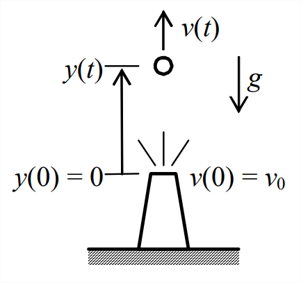
Figure \(\PageIndex{1}\) - First, let us idealize the aerodynamic drag force as being linearly viscous with damping constant \(c\), \(D_1\) = \(cv\) (subscript 1 denotes this mathematical model of drag as proportional to the 1st power of velocity, \(v^1\)). Draw and label an appropriate free-body diagram (FBD), showing the direction of drag force, by convention in analysis of aerodynamics, as being opposite to the direction of velocity \(v(t)\). Using your FBD, apply Newton’s 2nd law to derive the ODE of motion, \(m\dot{v} + cv = mg\).2
- Solve the ODE of part (a) to determine an equation for velocity \(v(t)\), \(t\) \(\geq\) 0, given the known IC, \(v(0)\) = \(v_0\). First, observe that the homogeneous ODE is the same as Equation 1.5.3, so that Equation 1.5.6 is the homogeneous solution. Next, find the simplest possible particular solution, \(v_p\), a constant. Next, enforce the initial condition to determine the unknown constant of the homogeneous solution. From your \(v(t)\) equation, show that \(v_p\) = \(v_{t1}\), the constant terminal velocity of the ball’s descent for drag \(D_1\). Also, derive an equation for the instant of time \(t_z{1}\) when velocity is zero, which, of course, corresponds to the peak altitude, \(y_{max\_1}\) of the ball. (Partial answers: \(V_{t1}\) = \(-mg/c\); \(t_{z1}\) = \((m/c)\ln(1-v_0/v_{t1})\), in which \(\ln\) denotes the natural logarithm, i.e., the logarithm to base \(e\).)
- Integrate \(v(t)\) of part 1.7.2 to derive an equation for the ball’s altitude, \(y(t)\), \(t\) \(\geq\) 0; define the launch point to be the reference position, i.e., set the IC as \(y(0)\) ≡ 0. (Answer: \(y(t)\) = \((m/c)(v_0-v_{t1})(1-e^{-(c/m)t})+v_{t1}t\).)
- Next, let us consider the mathematical model for the aerodynamic drag force that is generally considered most appropriate for a smooth ball: \(D_2\) = \(\pm \bar{q} S C_{D}\), with the plus sign for ascent (\(v\) \(\geq\) 0), and the minus sign for descent (\(v\) < 0). The terms in this equation are: \(\bar{q}=\frac{1}{2} \rho v^{2}\), the dynamic pressure, with sea-level air density \(\rho\) = 0.002 377 slug/ft3 = 0.002 377 lb-s2/ft4 ; \(S=\pi d^{2} / 4\), the ball’s projected area, with baseball diameter about \(d\) = 2.90 inches; and \(C_D\), the dimensionless drag coefficient, which is about \(C_D\) = 0.50 for the smooth ball, provided its airspeed is less than about 140 mph (miles/hour). Write two 1st order ODEs for \(v(t)\) with drag model \(D_2\), one ODE applying to ascent, the other to descent. Explain what it is about these ODEs that makes them nonlinear. Do not attempt to solve these ODEs in general, but use the appropriately simplified form of the descent ODE to find an algebraic equation for \(v_{t2}\), the constant terminal velocity of the ball’s descent for drag \(D_2\); and then calculate the value of \(v_{t2}\) in mph. Use the average weight of baseballs, \(m g\) = \(5\frac{1}{8}\) ounces, with \(g\) = 32.17 ft/s2 . Note: 60 mph = 88 ft/s, 1 foot = 12 inches, and 1 lb = 16 ounces. (Partial answer: \(v_{t2}\) = −74.91 mph. It might seem counterintuitive that the terminal velocity of a stitched baseball is −95 mph, a much greater speed than that of an otherwise equivalent smooth ball; see Adair, 1994, pages 5-12.3)
- Let us attempt to establish some sort of “equivalent” linear mathematical model relative to the nonlinear model of part 1.7.4. The only comparable results that we have determined for this purpose are the equations for terminal velocity. Therefore, calculate an “equivalent” linear viscous damping constant \(c\) by equating \(v_{t1}\) = \(v_{t2}\). Suppose that \(v_0\)= 110 mph, the average speed at which a baseball rebounds from a bat on the ball’s way to a 400-foot major league home run. Calculate the total ascent time \(t_{z1}\) (in seconds) and the peak altitude \(y(t_{z1})\) ≡ \(y_{max\_1}\) (in feet), quantities that are defined in parts 1.7.2 and 1.7.3. It happens that both nonlinear ODEs of part 1.7.4 can be solved in terms of standard mathematical functions.4 In particular, solution of the nonlinear ODE for ascent leads to the equation for total ascent time, \(t_{z 2}=\left[\left(-v_{t 2}\right) / g\right] \tan ^{-1}\left[v_{0} /\left(-v_{t 2}\right)\right]\), and the equation for peak altitude, \(y\left(t_{z 2}\right) \equiv y_{\max _{2}}=\left(v_{t 2}^{2} / g\right) \ln \sqrt{1+\left(v_{0} / v_{t 2}\right)^{2}}\). Calculate \(t_{z2}\) and \(y_{max\_2}\), and compare them, respectively, with \(t_{z1}\) and \(y_{max\_1}\); note, however, that we cannot infer from this limited comparison the general quality of the “equivalent” linear model relative to the nonlinear model. (Partial answers: \(c\) = 2.955 \(\times\) 10-3 lb-s/ft; \(y_{max\_1}\) = 210.7 ft; \(t_{z2}\) = 3.299 sec)
- The ODE solution procedure illustrated in Section 1-5 for a 1st order ODE can be used to solve any LTI ODE or system of LTI ODEs. Consider, for example, the 2nd order ODE Equation 1.9.6 for a mass-damper-spring system, \(m \ddot{x}+c \dot{x}+k x=f_{x}(t)\). The physical parameters \(m\), \(c\), and \(k\) are known constants.
- Seek a homogeneous solution in the form \(x_{h}(t)=C e^{\lambda t}\) as follows. First, show that the characteristic equation is a quadratic polynomial in the unknown \(\lambda\). Next, solve the polynomial equation and show in detail that there are two characteristic values (roots), \(\lambda_{1,2}=-\frac{c}{2 m} \pm \sqrt{\left(\frac{c}{2 m}\right)^{2}-\frac{k}{m}}\). Assume that \(\left(\frac{c}{2 m}\right)^{2}>\frac{k}{m}\). Therefore, the general homogeneous solution must have the form \(x_{h}(t)=C_{1} e^{\lambda_{1} t}+C_{2} e^{\lambda_{2} t}\), with two initially unknown constants.
- Suppose that the excitation force has the sinusoidal form \(f_{x}(t)=F \sin \omega t\), in which force amplitude \(F\) and circular frequency \(\omega\) (in radians/second) are considered to be known. Seek a particular solution by using the method of undetermined coefficients. First, express the solution as \(x_{p}(t)=P_{1} \sin \omega t+P_{2} \cos \omega t\). Now, substitute this into the non-homogeneous ODE to find algebraic equations for and in terms of the constants that \(m\), \(c\), \(k\), \(F\), and \(\omega\). (Partial answer: \(P_{2}=\frac{-c \omega}{\left(k-m \omega^{2}\right)^{2}+(c \omega)^{2}} F\))
- Express the complete solution as \(x(t)=x_{h}(t)+x_{p}(t)\). Suppose that the mass \(m\) is initially at rest with ICs: initial position \(x(0) = 0\) and initial velocity \(\dot{x}(0)=0\). Use these ICs to write two linear equations with unknowns \(C_1\) and \(C_2\). Solve for \(C_1\) and \(C_2\); show that they can be written as \(C_{1}=\frac{P_{2} \lambda_{2}-P_{1} \omega}{\lambda_{1}-\lambda_{2}}\) and \(C_{2}=\frac{P_{1} \omega-P_{2} \lambda_{1}}{\lambda_{1}-\lambda_{2}}\).
Note that a reasonably efficient algebraic equation for the final result \(x(t)\) is derived by defining constants \(C_1\) and \(C_2\) in terms of the previously defined \(\lambda_i\) and \(P_i\), rather than writing them in terms of all the basic parameters, \(m\), \(c\), \(k\), \(F\), and \(\omega\).
- Solve Problem 1.8 in MATLAB. Begin with the following MATLAB commands:
>> syms x t m c k F w>> x=dsolve('D2x+c/m*Dx+k/m*x=F/m*sin(w*t)','x(0)=0','Dx(0)=0')The MATLAB response will probably be an equation for \(x(t)\) of truly breathtaking length. You can try simplification operations such as
x=simple(x)andpretty(x)and thesubexprcommand, but they will not necessarily lead to a more useful equation for \(x(t)\). At some point, you might decide that, rather than continuing to flail away at the symbolic software, your time is used more efficiently if you just solve by hand and define intermediate symbols in terms of the basic parameters, as is done in Problem 1.8. - This problem relates to the details of the mass-spring-system ODE solution presented in Section 1-10.
- Substitute the assumed particular solution Equation 1.10.6 into non-homogeneous ODE Equation 1.10.5, then carry out the process in all algebraic detail to verify Equations 1.10.7 for \(P_1\) and \(P_2\).
- Substitute ICs Equation 1.10.2, \(\dot{x}(0)=0\) and \(x(0)=0\) into complete solution Equation 1.10.9, then carry out the process in all algebraic detail to verify Equations 1.10.10 for \(C_1\) and \(C_2\).
- Consider a mass-spring system with an “exponential step” forcing function, as described by the 2nd order LTI ODE \(m \ddot{x}+k x=f_{x}(t)=F\left(1-e^{-t / t_{c}}\right)\), in which position \(x(t)\) is the dependent variable, and the known constant parameters are mass \(m\), spring stiffness constant \(k\), force amplitude \(F\), and time constant \(t_c\). The time constant is the time required for the “exponential unit-step” function, \(1-e^{-t / t_{c}}\), to rise from 0 at \(t\) = 0 to the value \(1-e^{-1}\) = 0.6321, on its way to the asymptotic value 1 as \(t\rightarrow\inf\).
- Use the method of undetermined coefficients to derive an algebraic equation (in terms of the given constants) for the particular solution \(x_p(t)\) of this ODE and forcing function.
- Let the ICs for this \(m\)-\(k\) system be \(\dot{x}(0)=0\) and \(x(0)=0\). Use the result of part (a) and whatever else is required to derive in all detail the following complete algebraic solution for \(x(t)\), \(t\) \(\geq\) 0, in which \(\omega_{n}=\sqrt{k / m}\): \[x(t)=\frac{F}{k}\left\{1-\frac{1}{1+\left(1 / \omega_{n} t_{c}\right)^{2}}\left[e^{-t / t_{c}}+\left(1 / \omega_{n} t_{c}\right) \sin \omega_{n} t+\left(1 / \omega_{n} t_{c}\right)^{2} \cos \omega_{n} t\right]\right\} \nonumber \]
- Consider the specific numerical case of mass \(m\) = 8.03 kg, spring stiffness constant \(k\) = 317 N/m, and force amplitude \(F\) = 4.50 N. Calculate the circular natural frequency \(\omega_n\) and the cyclic natural frequency \(f_n\). Let excitation time constant \(t_{c}=1 / \omega_{n}\), a much shorter interval than the \(m\)-\(k\) system’s natural period \(T_{n}=2 \pi / \omega_{n}\). Compose and run a MATLAB program that does the following: calculate the actual dynamic response \(x(t)\) and the pseudo-static response \(f_{x}(t) / k\) over the time interval 0 \(\leq\) \(t\) \(\leq\) 2.5 s; plot both \(x(t)\) and \(f_{x}(t) / k\) on the same graph in units of either centimeters or millimeters. Explain in a sentence or two what feature of your plot of \(x(t)\) demonstrates and conforms with your calculation of \(f_n\).
- Consider a mass-spring system with a sinusoidal forcing function, as described by the 2nd order LTI ODE \(m \ddot{x}+k x=f_{x}(t)=F \sin \omega t\), in which position \(x(t)\) is the dependent variable, and the known constant parameters are mass \(m\), spring stiffness constant \(k\), force amplitude \(F\), and excitation frequency \(\omega\).
- Use the method of undetermined coefficients to derive an algebraic equation (in terms of the given constants) for the particular solution \(x_p(t)\) of this ODE and forcing function, a solution that is valid provided \(\omega^{2} \neq k / m\).
- Let the ICs for this \(m\)-\(k\) system be \(\dot{x}(0)=0\) and \(x(0)=0\). Use the result of part 1.12.1 and whatever else is required to derive in all detail the following complete algebraic solution for \(x(t)\), \(t\) \(\geq\) 0, in which \(\omega_{n}=\sqrt{k / m}\): \[x(t)=\frac{F}{k} \frac{1}{1-\left(\omega / \omega_{n}\right)^{2}}\left[\sin \omega t-\left(\omega / \omega_{n}\right) \sin \omega_{n} t\right], \text { valid for } \omega \neq \omega_{n} \nonumber \]
- Consider the specific numerical case of mass \(m\) = 0.230 lb-s2 /inch (which weighs about 88.8 lb), spring stiffness constant \(k\) = 227 lb/inch, and force amplitude \(F\) = 45.0 lb. Calculate the circular natural frequency ωn and the cyclic natural frequency \(f_n\). For excitation frequency \(\omega=1.2 \omega_{n}\), compose and run a MATLAB program that does the following: calculate the actual dynamic response \(x(t)\) and the pseudo-static response \(f_{x}(t) / k\) over the time interval 0 \(\geq\) \(t\) \(\geq\) 2 s; plot both \(x(t)\) and \(f_{x}(t) / k\) on the same graph. Your \(x(t)\) plot should exhibit the phenomenon of beating, which is analyzed more completely in Section 10-6.
- The \(x(t)\) equation derived in part 1.12.2 is not valid if excitation frequency \(\omega\) equals natural frequency \(\omega_n\), but note that in this case the \(x(t)\) equation has the indeterminate form 0/0, so that we can apply l’Hospital’s rule (which is described in any calculus textbook) to find the limit-case response solution. Define \(\beta=\omega / \omega_{n}\), so that \(\omega t=\beta \omega_{n} t\). Now, hold \(\omega_n\) constant and take the limit as \(\beta \rightarrow 1\) of the \(x(t)\) equation in order to determine the correct response \(x(t)\) equation for the case \(\omega=\omega_{n}\).
1Mathematica ® is a registered trademark of Wolfram Research, Inc.
2In Appendix B, Section B-2, this ODE is derived by an alternative method using energy and power.
3Literature references such as this are described in detail in the References section following Chapter 17.
4For examples of these solutions, see: an ascent solution in Greenwood, 1965, Problem 3-4 on pages 128 and 503; and a descent solution in Sommerfeld, 1964, pages 21-22.