4.8: Chapter 4 Homework
- Page ID
- 7980
\( \newcommand{\vecs}[1]{\overset { \scriptstyle \rightharpoonup} {\mathbf{#1}} } \)
\( \newcommand{\vecd}[1]{\overset{-\!-\!\rightharpoonup}{\vphantom{a}\smash {#1}}} \)
\( \newcommand{\dsum}{\displaystyle\sum\limits} \)
\( \newcommand{\dint}{\displaystyle\int\limits} \)
\( \newcommand{\dlim}{\displaystyle\lim\limits} \)
\( \newcommand{\id}{\mathrm{id}}\) \( \newcommand{\Span}{\mathrm{span}}\)
( \newcommand{\kernel}{\mathrm{null}\,}\) \( \newcommand{\range}{\mathrm{range}\,}\)
\( \newcommand{\RealPart}{\mathrm{Re}}\) \( \newcommand{\ImaginaryPart}{\mathrm{Im}}\)
\( \newcommand{\Argument}{\mathrm{Arg}}\) \( \newcommand{\norm}[1]{\| #1 \|}\)
\( \newcommand{\inner}[2]{\langle #1, #2 \rangle}\)
\( \newcommand{\Span}{\mathrm{span}}\)
\( \newcommand{\id}{\mathrm{id}}\)
\( \newcommand{\Span}{\mathrm{span}}\)
\( \newcommand{\kernel}{\mathrm{null}\,}\)
\( \newcommand{\range}{\mathrm{range}\,}\)
\( \newcommand{\RealPart}{\mathrm{Re}}\)
\( \newcommand{\ImaginaryPart}{\mathrm{Im}}\)
\( \newcommand{\Argument}{\mathrm{Arg}}\)
\( \newcommand{\norm}[1]{\| #1 \|}\)
\( \newcommand{\inner}[2]{\langle #1, #2 \rangle}\)
\( \newcommand{\Span}{\mathrm{span}}\) \( \newcommand{\AA}{\unicode[.8,0]{x212B}}\)
\( \newcommand{\vectorA}[1]{\vec{#1}} % arrow\)
\( \newcommand{\vectorAt}[1]{\vec{\text{#1}}} % arrow\)
\( \newcommand{\vectorB}[1]{\overset { \scriptstyle \rightharpoonup} {\mathbf{#1}} } \)
\( \newcommand{\vectorC}[1]{\textbf{#1}} \)
\( \newcommand{\vectorD}[1]{\overrightarrow{#1}} \)
\( \newcommand{\vectorDt}[1]{\overrightarrow{\text{#1}}} \)
\( \newcommand{\vectE}[1]{\overset{-\!-\!\rightharpoonup}{\vphantom{a}\smash{\mathbf {#1}}}} \)
\( \newcommand{\vecs}[1]{\overset { \scriptstyle \rightharpoonup} {\mathbf{#1}} } \)
\(\newcommand{\longvect}{\overrightarrow}\)
\( \newcommand{\vecd}[1]{\overset{-\!-\!\rightharpoonup}{\vphantom{a}\smash {#1}}} \)
\(\newcommand{\avec}{\mathbf a}\) \(\newcommand{\bvec}{\mathbf b}\) \(\newcommand{\cvec}{\mathbf c}\) \(\newcommand{\dvec}{\mathbf d}\) \(\newcommand{\dtil}{\widetilde{\mathbf d}}\) \(\newcommand{\evec}{\mathbf e}\) \(\newcommand{\fvec}{\mathbf f}\) \(\newcommand{\nvec}{\mathbf n}\) \(\newcommand{\pvec}{\mathbf p}\) \(\newcommand{\qvec}{\mathbf q}\) \(\newcommand{\svec}{\mathbf s}\) \(\newcommand{\tvec}{\mathbf t}\) \(\newcommand{\uvec}{\mathbf u}\) \(\newcommand{\vvec}{\mathbf v}\) \(\newcommand{\wvec}{\mathbf w}\) \(\newcommand{\xvec}{\mathbf x}\) \(\newcommand{\yvec}{\mathbf y}\) \(\newcommand{\zvec}{\mathbf z}\) \(\newcommand{\rvec}{\mathbf r}\) \(\newcommand{\mvec}{\mathbf m}\) \(\newcommand{\zerovec}{\mathbf 0}\) \(\newcommand{\onevec}{\mathbf 1}\) \(\newcommand{\real}{\mathbb R}\) \(\newcommand{\twovec}[2]{\left[\begin{array}{r}#1 \\ #2 \end{array}\right]}\) \(\newcommand{\ctwovec}[2]{\left[\begin{array}{c}#1 \\ #2 \end{array}\right]}\) \(\newcommand{\threevec}[3]{\left[\begin{array}{r}#1 \\ #2 \\ #3 \end{array}\right]}\) \(\newcommand{\cthreevec}[3]{\left[\begin{array}{c}#1 \\ #2 \\ #3 \end{array}\right]}\) \(\newcommand{\fourvec}[4]{\left[\begin{array}{r}#1 \\ #2 \\ #3 \\ #4 \end{array}\right]}\) \(\newcommand{\cfourvec}[4]{\left[\begin{array}{c}#1 \\ #2 \\ #3 \\ #4 \end{array}\right]}\) \(\newcommand{\fivevec}[5]{\left[\begin{array}{r}#1 \\ #2 \\ #3 \\ #4 \\ #5 \\ \end{array}\right]}\) \(\newcommand{\cfivevec}[5]{\left[\begin{array}{c}#1 \\ #2 \\ #3 \\ #4 \\ #5 \\ \end{array}\right]}\) \(\newcommand{\mattwo}[4]{\left[\begin{array}{rr}#1 \amp #2 \\ #3 \amp #4 \\ \end{array}\right]}\) \(\newcommand{\laspan}[1]{\text{Span}\{#1\}}\) \(\newcommand{\bcal}{\cal B}\) \(\newcommand{\ccal}{\cal C}\) \(\newcommand{\scal}{\cal S}\) \(\newcommand{\wcal}{\cal W}\) \(\newcommand{\ecal}{\cal E}\) \(\newcommand{\coords}[2]{\left\{#1\right\}_{#2}}\) \(\newcommand{\gray}[1]{\color{gray}{#1}}\) \(\newcommand{\lgray}[1]{\color{lightgray}{#1}}\) \(\newcommand{\rank}{\operatorname{rank}}\) \(\newcommand{\row}{\text{Row}}\) \(\newcommand{\col}{\text{Col}}\) \(\renewcommand{\row}{\text{Row}}\) \(\newcommand{\nul}{\text{Nul}}\) \(\newcommand{\var}{\text{Var}}\) \(\newcommand{\corr}{\text{corr}}\) \(\newcommand{\len}[1]{\left|#1\right|}\) \(\newcommand{\bbar}{\overline{\bvec}}\) \(\newcommand{\bhat}{\widehat{\bvec}}\) \(\newcommand{\bperp}{\bvec^\perp}\) \(\newcommand{\xhat}{\widehat{\xvec}}\) \(\newcommand{\vhat}{\widehat{\vvec}}\) \(\newcommand{\uhat}{\widehat{\uvec}}\) \(\newcommand{\what}{\widehat{\wvec}}\) \(\newcommand{\Sighat}{\widehat{\Sigma}}\) \(\newcommand{\lt}{<}\) \(\newcommand{\gt}{>}\) \(\newcommand{\amp}{&}\) \(\definecolor{fillinmathshade}{gray}{0.9}\)- This problem involves the data and results for the 1st order damper-spring system that is analyzed in Section 4.2 with use of MATLAB program
MATLABdemo41.- Substitute the damper-spring data and the given values of \(F\) and \(\omega\) into Equation 4.3.8 and 4.3.10 in order to calculate the magnitude \(X\) and phase angle φ (in degrees, in the range −180° \(\leq\) \(\phi\) < +180°) of the frequency response.
- Examine the time history graph generated by MATLAB program
MATLABdemo41. The purpose of this problem is for you to evaluate that graph as if it were recorded from an experiment. Consider, in particular, the time after about \(t\) = 1.3 s, when the output has settled into steady-state sinusoidal response. Measure from the graph the steady-state output magnitude \(X\). Measure whatever information is required from the graph, then calculate phase angle \(\phi\) (in degrees, in the range −180° \(\leq\) \(\phi\) < +180°) of the steady-state state response. These simulated experimental results for \(X\) and \(\phi\) should be equal to (or at least close to, since it is not possible to make precise measurements from a graph) the comparable results calculated in part 1.1 from theoretical formulas.
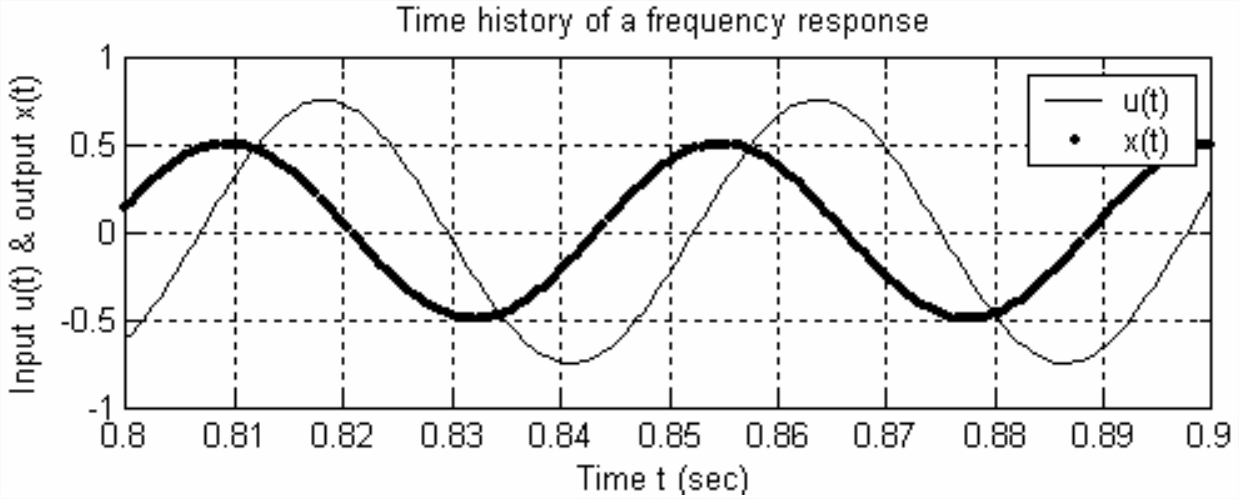
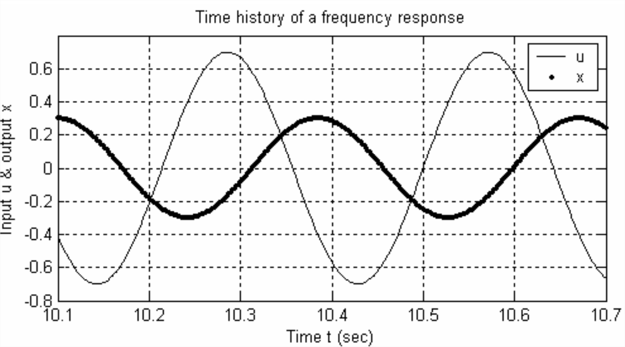
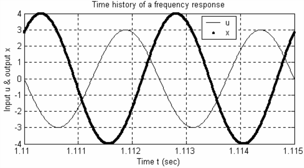
- An experimental frequency response test is conducted on an LTI system (not necessarily a 1st order system), with input \(u(t)=U \cos \omega t\) and output \(x(t)=X \cos (\omega t+\phi)\). A simulated graph [2.1 or 2.2 or 2.3, whichever is assigned] of the steady-state input and output quantities at one particular frequency is shown below or on the next page. Calculate from the graph, with as much accuracy as the data permits, the following values: (i) the sinusoidal period \(T_p\), and then the frequency (in both Hz and rad/s), (ii) the FRF magnitude ratio \(X / U\) (assume consistent physical units), and (iii) the FRF phase \(\phi\) (in degrees, in the range −180° \(\leq\) \(\phi\) < +180°).
-

Figure \(\PageIndex{1}\) -

Figure \(\PageIndex{2}\) -

Figure \(\PageIndex{3}\)
-
- The governing ODE of the series damper-spring low-pass filter in Figure 3.7.4 is Equation 3.7.5, \(\tau_{1} \dot{x}_{o}+x_{o}=x_{i}(t)\). Show that the associated 1st order complex frequency-response function is \(F R F(\omega)=T F(j \omega)=1 /\left(1+j \omega \tau_{1}\right)\). The following MATLAB script graphs from this equation the FRF magnitude ratio and phase in one conventional format (log-log for magnitude ratio, semilog for phase in degrees, magnitude ratio graph directly over phase graph), for the case of time constant \(\tau_{1}\) = 0.0145 s, with excitation frequencies ranging from 1 Hz to 1 000 Hz. Note that MATLAB does most of the work for you if you start with the complex FRF, and then use MATLAB’s capability for performing complex arithmetic. In particular, the MATLAB function
abscalculates the absolute value (magnitude) of a complex number, and the MATLAB functionanglecalculates the angle in radians of a complex number.t1=0.0145; % First-order system time constant (sec)f=logspace(0,3,200);w=2*pi*f; % 200 pts. 1 Hz-1 kHz evenly spaced on log scaleFRF=1./(1+j*w*t1); % complex FRF; note necessity of array operation ./magrat=abs(FRF);fazdeg=angle(FRF)*180/pi; % magnitude ratio and phase in degsubplot(2,1,1),loglog(f,magrat,'k'),grid,ylabel('FRF magnitude ratio'), ...title('FRF of 1st order system with time constant = 0.0145 sec')subplot(2,1,2),semilogx(f,fazdeg,'k'),grid, ...ylabel('FRF phase (deg)'),xlabel('Frequency (Hz)')Run this script on your computer, and submit the graphs that it produces. Additionally,
- calculate the break frequency \(f_{b}=1 /\left(2 \pi \tau_{1}\right)\) and show that it matches the break frequency inferred from the MATLAB graphs;
- use complex arithmetic to evaluate by hand (and hand calculator) the complex FRF, \(F R F(\omega)=\frac{1}{1+j \omega \tau_{1}}\), at frequency \(f\) = 30 Hz, and show that your hand-calculated magnitude ratio and phase match those of MATLAB. You might have occasion to do more graphing of FRFs, so, for your future reference, make sure that you understand the operations of all the MATLAB commands in the above script.
- The governing ODE of the series damper-spring high-pass filter in Figure 3.7.4 is Equation 3.7.6, \(\dot{x}_{o}+\left(1 / \tau_{1}\right) x_{o}=\dot{x}_{i}(t)\) [see also homework Problem 3.7].
- Show that the associated 1st order high-pass filter complex frequency-response function is \(F R F(\omega)=j \omega \tau_{1} /\left(1+j \omega \tau_{1}\right)\).
- For frequency response, we are evaluating the input in the form \(x_{i}(t)=X_{i} \cos \omega t\) and the output in the form \(x_{o}(t)=X_{o} \cos (\omega t+\phi)\). Use the FRF of part 4.1 to show that the equations for FRF magnitude ratio and phase are \[\frac{X_{o}(\omega)}{X_{i}}=\frac{\omega \tau_{1}}{\sqrt{1+\left(\omega \tau_{1}\right)^{2}}}, \quad \phi(\omega)=\frac{\pi}{2}-\tan ^{-1}\left(\omega \tau_{1}\right)=\tan ^{-1}\left(\frac{1}{\omega \tau_{1}}\right) \nonumber \] Use this magnitude ratio equation to derive equations for the low-frequency and high-frequency asymptotes, and sketch those asymptotes on a log-log graph such as Figure 4.3.3. You may use the definition of break frequency, \(\omega_{b}=1 / \tau_{1}\), so that \(\omega \tau_{1}=\omega / \omega_{b}=f / f_{b}\). This system has the character of a mild high-pass filter, so your sketch of the asymptotes should have the appearance appropriate to that name.
- Let the time constant \(\tau_{1}\) = 1 s, and consider the excitation frequency range 0.01 \(\leq\) \(\omega\) \(\leq\) 100 rad/s (10-2 \(\leq\) \(\omega\) \(\leq\) 10+2 rad/s). Adapt the MATLAB program, and use the graphical format provided in homework Problem 4.3 to graph with MATLAB the FRF magnitude ratio and phase (in degrees). As is done in Problem 4.3, program directly the complex FRF, in this case \(F R F(\omega)=j \omega \tau_{1} /\left(1+j \omega \tau_{1}\right)\), not the equations of part 4.4.3.
- A standard LTI mass-damper-spring system has the ordinary differential equation of motion \(m \ddot{x}+c \dot{x}+k x=f_{x}(t)\), in which \(f_{x}(t)\) is the input and \(x(t)\) is the output.
- Use the ODE to derive the transfer function \(T F(s) \equiv L[x(t)]_{I C s=0} / L\left[f_{x}(t)\right]\) for the \(m\)-\(c\)-\(k\) system. This transfer function is an algebraic equation in terms of independent variable \(s\) and constants \(m\), \(c\), and \(k\).
- Use transfer function \(TF(s)\) to derive the complex frequency-response function \(FRF(\omega)\) for the \(m\)-\(c\)-\(k\) system in terms of independent variable frequency \(\omega\) and constants \(m\), \(c\), and \(k\).
- From \(FRF(\omega)\) for the \(m\)-\(c\)-\(k\) system, write equations in terms of independent variable frequency \(\omega\) and constants \(m\), \(c\), and \(k\) for the real magnitude ratio \(|F R F(\omega)|\) and the real phase angle \(\angle F R F(\omega)=\phi(\omega)\).


