11.4: Chapter 4 Homework

1. The trimming tab of a small airplane is attached to the elevator by a hinge at axis \(H\) and a rotational spring (the actuator linkage) with constant \(k_{\theta}\), as shown in the drawing below. You are required to determine experimentally both rotational inertia \(J_H\) of the elevator about the hinge, and rotational stiffness \(k_{\theta}\). The field experiment consists of two separate twang tests. (See homework Problem 9.4 for a detailed description of twang testing and relevant equations.) First, the rotational spring is disconnected from the tab, and a vertical translational support spring of known stiffness \(k_y = 15.6\) lb/inch (and low mass, producing negligible inertial force) is attached near the trailing edge, as shown. Then the tab is twanged (displaced statically from the static equilibrium position, then released). A non-contacting displacement sensor picks up the dynamic motion at a point near the support spring: \(y(t)=0.107 e^{-0.144 t} \cos (59.9 t)\) inch (\(t\) in seconds). (There is slight damping due to friction at the hinge, internal structural damping in the spring, and drag of the surrounding air.) From this first twang test, calculate \(J_H\) (in lb-s² -inch). Next, translational spring \(k_y\) is removed, rotational spring \(k_{\theta}\) is re-connected, and the tab is again twanged. The same displacement sensor as in the first twang test now measures dynamic motion \(y(t)=0.132 e^{-0.112 t} \cos (66.0 t)\) inch. From the previous results and this second twang test, calculate \(k_{\theta}\) (in lb-inch/radian).

   

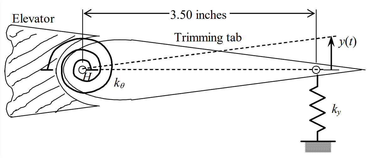
   Figure \(\PageIndex{1}\)

2. The system depicted on the next page consists of a rigid bar, a mass, and springs. The rigid bar is supported at frictionless hinge \(H\), where it is elastically restrained by rotational spring \(k_{\theta}\), and the rotational inertia of the bar about point \(H\) is \(J_{H}\). Mass \(m\) is connected to the bar by translational spring \(k_y\) at point \(B\), and the mass is restrained to move only vertically by frictionless walls. An externally applied vertical force \(F(t)\) acts on the bar at point \(B\). Degrees of freedom \(y(t)\) and \(\theta(t)\) are the small motions relative to the static equilibrium position. Sketch and label a DFBD for the bar and a DFBD for mass \(m\), then use these diagrams to derive the two coupled differential equations of motion for this system. (Hints: Show that for small bar rotation, the stretch of spring \(k_y\) is \(a \theta-y\). Do not include \(mg\) or bar weight among the applied forces, because we are interested only in dynamic motions relative to the static equilibrium position; if you are not sure why we neglect weights in these equations of motion, then review Section 7.5.)

   

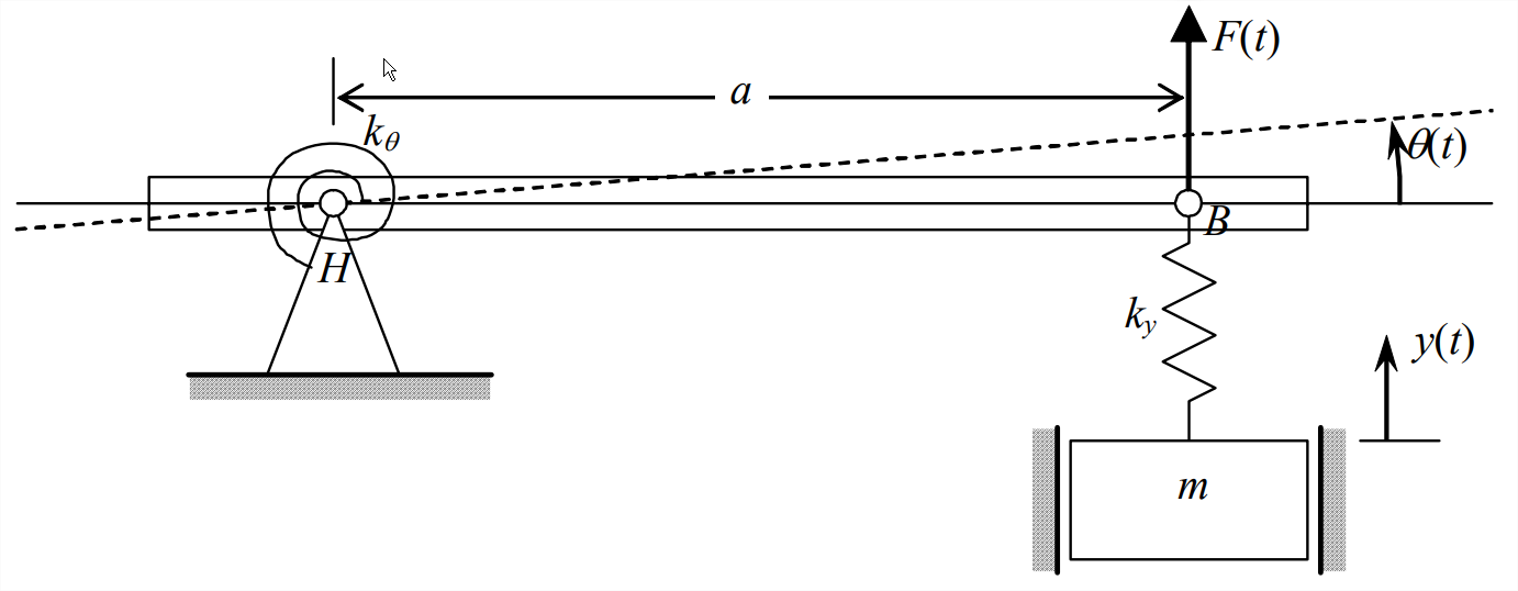
   Figure \(\PageIndex{2}\)

3. The two-degrees-of-freedom system drawn below consists of a pendulum supported at frictionless hinge \(H\), and a mass-spring connected by a viscous damper to the pendulum rod. The inertial moment of the lightweight pendulum rod is negligible, so pendulum rotational inertia about \(H\) is \(J_{H}=m_{p} \ell^{2}\). Degrees of freedom \(x(t)\) and \(\theta(t)\) are \(m\) small motions relative to the static equilibrium position. Show that the velocity of the damper cylinder relative to the damper piston is \(\dot{x}-a \dot{\theta}\). Both gravity and the externally applied horizontal force \(F(t)\) act on mass \(m_{p}\) of the pendulum bob. Sketch and label an FBD for the pendulum and an FBD for mass \(m\), then use these diagrams to derive the two coupled differential equations of motion for this system. In addition to the motion and force variables and the constant parameters shown on the drawing, the acceleration of gravity acting vertically downward is denoted \(g\). For this problem, unlike for Problems 11.1 and 11.2 and the examples in Section 11.3, you should sketch your pendulum FBD with the pendulum rotated through a small angle, so that you can indicate the restraining effect of weight \(m_pg\) on pendulum rotation; see the pendulum example in Section 7.1.

   

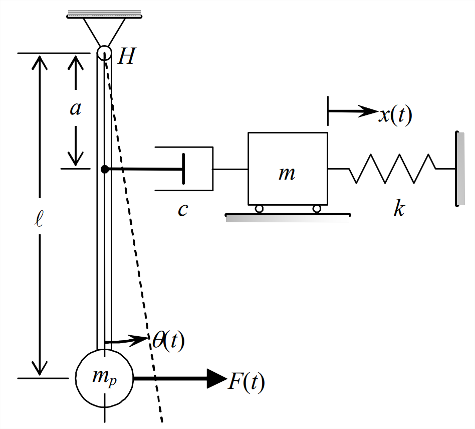
   Figure \(\PageIndex{3}\)

4. The form of the typical-section ODEs of motion represented by Equations 11.3.14, 11.3.15, and 11.3.16 is not unique. Suppose, for example, you want to define \(y_{E A}(t)\) as the vertical translation degree of freedom, instead of \(y_{c}(t)\). With use of geometry, inertia, and algebraic manipulation, you can cast the ODEs into a cosmetically different, but mathematically equivalent form. First, substitute Equation 11.3.11 into Equations 11.3.14 and 11.3.15 in order to replace \(y_{c}(t)\) with appropriate terms that include \(y_{E A}(t)\) and small-rotation \(\theta(t)\); next, use the parallel-axis theorem to replace \(J_{C}\) with the rotational inertia about the elastic axis, \(J_{E A}\), and a term including mass \(m\); finally, perform any additional algebraic substitution required to write the ODEs of motion in the following relatively simple matrix form:\[\overbrace{\left[\begin{array}{cc}
   m & m r \\
   m r & J_{E A}
   \end{array}\right]}^{\text {inertia matrix }}\left[\begin{array}{c}
   \ddot{y}_{E A} \\
   \ddot{\theta}
   \end{array}\right] + \overbrace{\left[\begin{array}{cc}
   k_{y} & 0 \\
   0 & k_{\theta}
   \end{array}\right]}^{\text {structural stiffness matrix }}\left[\begin{array}{c}
   y_{E A} \\
   \theta
   \end{array}\right] = \left[\begin{array}{c}
   F_{L}(t) \\
   e F_{L}(t)+M_{A C}(t)
   \end{array}\right] \nonumber \]Which terms in this matrix equation produce and display the coupling between vertical translation \(y_{E A}(t)\) and pitching rotation \(\theta(t)\)? Will this coupling still exist if the applied aerodynamic actions \(F_{L}(t)\) and \(M_{A C}(t)\) are either constant or vary slowly enough that the response is pseudo-static? Prove the positive definiteness of these inertia and structural stiffness matrices by finding the values and polarities of their determinants.
5. Consider the pendulum-spring system depicted below. The inertial moments of the lightweight pendulum rods are negligible, so pendulum rotational inertias about their hinges are \(J_{i}=m_{i} \ell^{2}\), \(i = 1, 2\). Degrees of freedom \(\theta_{1}(t)\) and \(\theta_{2}(t)\) are small rotations relative to the vertical hanging static equilibrium positions. A horizontal translational spring with stiffness constant \(k\) connects the two pendulums, and it is undeformed when the pendulums are in the vertical hanging static equilibrium positions. Show that the stretch of the spring is given by \(a\left(\theta_{2}-\theta_{1}\right)\). Externally applied moment \(M_{2}(t)\) acts on pendulum 2 at its hinge (applied, for example, by a motor). Sketch and label an FBD for each pendulum, then use these diagrams to derive the two coupled differential equations of motion for this system. In addition to the motion and applied action variables and the constant parameters shown on the drawing, the acceleration of gravity acting vertically downward is denoted \(g\). In this problem, you should sketch your FBDs with the pendulums rotated through small angles, so that you can indicate the restraining effect of the weights \(m_{i} g, i=1,2\), on the rotations; see the pendulum example in Section 7.1.

   

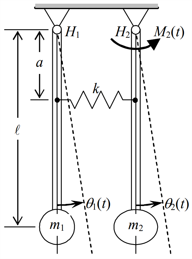
   Figure \(\PageIndex{4}\)

6. The drawing below depicts a very simplified model for the pitch-translation dynamics of an automotive vehicle. The body and frame are considered to be rigid, with center of mass \(C\) located as shown, and having mass \(m\) and rotational inertia \(J_C\) about \(C\). The wheel-axle assemblies are considered to have negligible inertial forces. The flexibilities of tires and suspension systems are lumped together into a single rear-axle translational spring \(k_1\) and a single front-axle translational spring \(k_2\). Damping is provided by shock struts and rubber tires, and it is lumped into viscous dashpots \(c_1\) and \(c_2\) arranged in parallel with the respective springs. Sketch and label a DFBD for this vehicle model, then use it to derive the two coupled differential equations of motion for this system, in terms of the given parameters. Use as degrees of freedom the small vertical translation \(y_{C}(t)\) and the small pitching rotation \(\theta(t)\), both relative to the static equilibrium position.

   

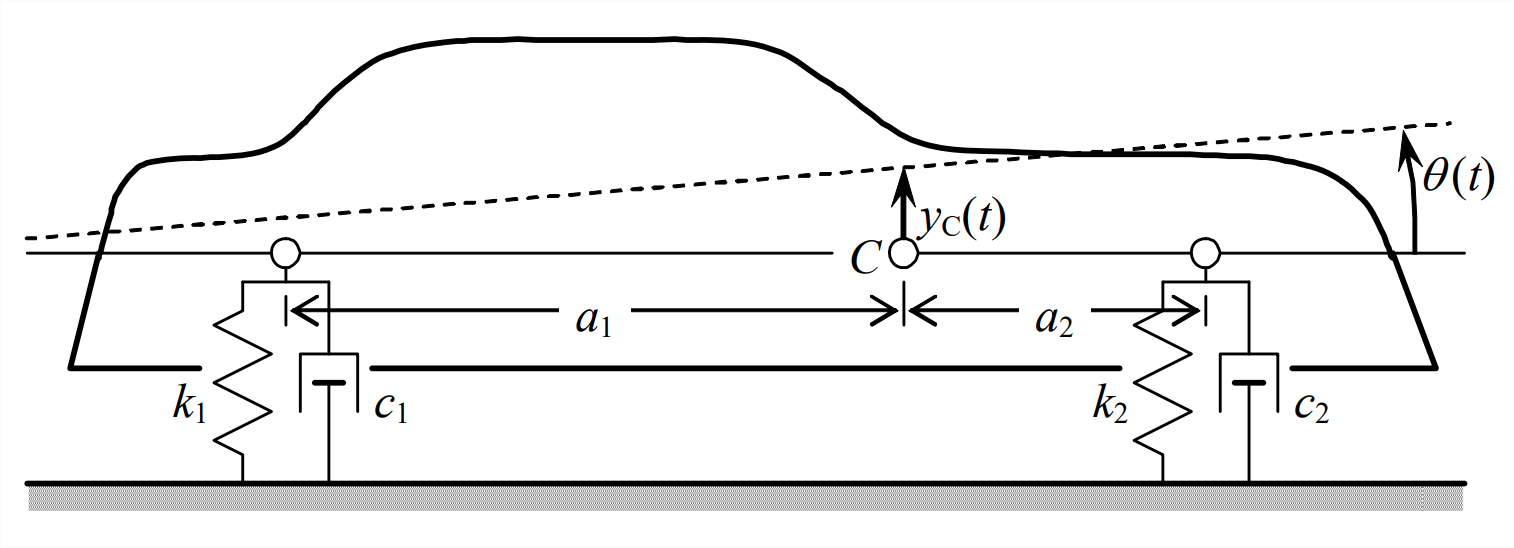
   Figure \(\PageIndex{5}\)