15.4: Example of PD Control

Next, we consider the effect of derivative control, the third type of operation on the error signal indicated in Equations 15.1.1 and 15.1.2. The derivative term (with \(b_{d}=1\)) in the actuator signal \(w(t)\) is \(P \tau_{d} \times d e_{e} / d t\). This term is proportional to the rate of change of the error signal, so it anticipates, in a sense, any increase in the error, and it acts to oppose that increase. Derivative action is used in combination with proportional action or proportional-integral action, but not by itself. Whereas proportional action has the effect of a restoring linear spring, derivative action has the effect of a viscous damper. Therefore, derivative control by itself would fail to provide action that forces system output toward the desired value.

A reality check is appropriate at this point. The derivative output \(x_{d}(t) \equiv \dot{e}_{e}\) of an ideal PID controller in Equation 15.1.1 is physically unrealistic, because it is not possible to measure exactly, in real time, the derivative \(\dot{e}_{e}\) of the error signal. Exact real-time measurement of a derivative at an instant would require information about e e& future values of the signal, but future values are unknown. Another manifestation of the unrealism of the derivative term is the associated transfer function, \(X_{d} / E_{e}=s / 1\), which is written here as a fraction on the right-hand side so as to emphasize that the polynomial order (in \(s\)) of the numerator is higher than that of the denominator. Thus, this transfer function is acausal, meaning that the current output of the ideal differentiator must be dependent upon future, as well as past and present, values of the error signal (see Bélanger, 1995, p. 440).

Since the exact differentiator of Equation 15.1.1 cannot be realized physically, an actual PD controller often includes an approximate differentiator in the form of a 1^st order high-pass filter described by the ODE \(\varepsilon \tau_{d} \dot{x}_{d}+x_{d}=\dot{e}_{e}\); in this ODE, \(\tau_{d}\) is the derivative time constant, and \(\mathcal{E}\) is a small positive number typically selected to be in the range 0.1 to 0.3 (Ogata, 2001, pages 700 and 727). The transfer function of this approximate differentiator is \(X_{d}(s) / E_{e}(s)=s /\left(\varepsilon \tau_{d} s+1\right)\), which is causal, therefore physically realizable. For error signals that are slowly varying in time relative to the high-pass-filter break frequency \(1 /\left(\varepsilon \tau_{d}\right)\) rad/s, this approximate differentiator is very accurate, but for faster error signals the device’s output fails to approximate the derivative of the error signal (see homework Problem 15.4). In practice, therefore, the selection of parameters \(\tau_{d}\) and \(\mathcal{E}\) is based at least partly on the speed of signals that the PD controller is expected to process. The operation of an actual PD controller using the approximate differentiator is \(w(t)=P\left[e_{e}(t)+\tau_{d} x_{d}(t)\right]\); you can easily show that the transfer function of the actual PD controller is

\[\frac{W(s)}{E_{e}(s)}=P\left(1+\tau_{d} \frac{X_{d}(s)}{E_{e}(s)}\right)=P\left(1+\frac{\tau_{d} s}{\varepsilon \tau_{d} s+1}\right)=P\left(\frac{(1+\varepsilon) \tau_{d} s+1}{\varepsilon \tau_{d} s+1}\right). \nonumber \]

It is standard in introductory discussions to describe PD control in the context of the ideal (though physically unrealizable) differentiator \(x_{d} \equiv \dot{e}_{e}\), rather than the more realistic approximate differentiator \(\mathcal{E} \tau_{d} \dot{x}_{d}+x_{d}=\dot{e}_{e}\). The approximate differentiator leads to a higher-order system and much more complicated algebra, from which it is difficult to infer basic physical characteristics of PD control. Therefore, in the rest of this section, and in the continued examination of this same example in homework Problem 15.1 and in Section 16.2, we shall follow the standard introductory procedure and use the ideal PD-controller transfer function \(P\left(1+\tau_{d} s\right)\) from Equation 15.1.2. Most of the theoretical results produced by this approach are good approximations to what would be realized from a properly designed real PD controller, at least for sufficiently slowly varying inputs and outputs.

Figure \(\PageIndex{1}\): Proportional control of rotor position. (Copyright; author via source)

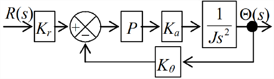
To illustrate proportional-derivative (PD) control, we consider again the problem of controlling position \(\theta(t)\) of a rotor with significant inertia \(J\), as discussed in Chapter 14 [Figures 14.1.1, 14.2.1, and 14.3.1, and Equations 14.1.1 and 14.1.2]. Recall that the input to the system is operator setting \(r(t)\). Let us neglect disturbance moments, \(M_{d}(t)=0\). Figure \(\PageIndex{1}\) is the Laplace block diagram for the P-controlled system, from which the loop transfer functions are \(G(s)=P K_{a} /\left(J s^{2}\right)\) and \(H(s)=K_{\theta}\). Hence, we use Equation 14.4.6 to find

\[C L T F(s)=\frac{\Theta(s)}{R(s)}=K_{r} \times \frac{N_{G} D_{H}}{D_{G} D_{H}+N_{G} N_{H}}=K_{r} \times \frac{P K_{a}}{J s^{2}+P K_{a} K_{\theta}} \equiv \frac{K_{r}}{K_{\theta}} \frac{\omega_{n}^{2}}{s^{2}+\omega_{n}^{2}} \nonumber \]

Undamped natural frequency in this \(\operatorname{CLTF}(s)\) is defined by \(\omega_{n}^{2}=P K_{a} K_{\theta} / J\). Suppose that the input is a step function with magnitude \(R_{H}: r(t)=R_{H} H(t)\). For this input, the Laplace transform of response is \(\Theta(s)=\frac{R_{H}}{s} \frac{K_{r}}{K_{\theta}} \frac{\omega_{n}^{2}}{s^{2}+\omega_{n}^{2}}\). Application of inverse transform Equation 15.2.23, with \(\zeta=0\), gives the step response \(\theta(t)=\left(R_{H} K_{r} / K_{\theta}\right)\left(1-\cos \omega_{n} t\right)\). This is undamped motion that oscillates forever about the desired final value, \(\theta=R_{H} K_{r} / K_{\theta}\) [see Equation 7.3.8 and Figure 7.3.2], so it is unacceptable for a position control system. In this case, P control alone has the effect of a restoring linear spring, but it provides no damping.

Figure \(\PageIndex{2}\): Ideal proportional-derivative (PD) control of rotor position. (Copyright; author via source)

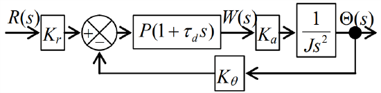
In order to improve the control performance, we add derivative action, upgrading from P control to ideal PD control. From Equation 15.1.2 with \(b_{i}=0\) and \(b_{d}=1\), the ideal PD-controller transfer function is \(P\left(1+\tau_{d} s\right)\), so the Laplace block diagram for the closed-loop system becomes that shown in Figure \(\PageIndex{2}\). In this case, the loop forward-branch transfer function is \(G(s)=P\left(1+\tau_{d} s\right) K_{a} /\left(J s^{2}\right)\), so the closed-loop transfer function of the system is

\[\frac{\Theta(s)}{R(s)}=K_{r} \times \frac{N_{G} D_{H}}{D_{G} D_{H}+N_{G} N_{H}}=K_{r} \times \frac{P\left(1+\tau_{d} s\right) K_{a}}{J s^{2}+P\left(1+\tau_{d} s\right) K_{a} K_{\theta}}=\frac{K_{r} P K_{a}\left(1+\tau_{d} s\right)}{J s^{2}+P K_{a} K_{\theta} \tau_{d} s+P K_{a} K_{\theta}} \nonumber \]

As we did in Equations 15.2.19 and 15.2.20, which apply to PI control (but of a different plant), we can now re-write this PD closed-loop transfer function in terms of parameters appropriate for a damped 2^nd order system:

\[\frac{\Theta(s)}{R(s)}=\frac{K_{r}}{K_{\theta}} \frac{\left(P K_{a} K_{\theta} / J\right)\left(\tau_{d} s+1\right)}{s^{2}+\left(P K_{a} K_{\theta} / J\right) \tau_{d} s+\left(P K_{a} K_{\theta} / J\right)} \equiv \frac{K_{r}}{K_{\theta}} \frac{\omega_{n}^{2}\left(\tau_{d} s+1\right)}{s^{2}+2 \zeta \omega_{n} s+\omega_{n}^{2}}\label{eqn:15.27} \]

In Equation \(\ref{eqn:15.27}\) the undamped natural frequency and the viscous damping ratio are, respectively:

\[\omega_{n}=\sqrt{\frac{P K_{a} K_{\theta}}{J}} \text { and } \zeta=\frac{1}{2 \omega_{n}} \frac{P K_{a} K_{\theta}}{J} \tau_{d}=\frac{1}{2} \omega_{n} \tau_{d}\label{eqn:15.28} \]

The obvious effect of the derivative action is to add damping to the 2^nd order system, and this damping improves the control performance (see homework Problem 15.1). Note also that the term \(\omega_{n}^{2} \tau_{d} S\) in the numerator of Equation \(\ref{eqn:15.27}\) makes this system non-standard relative to definition Equation 9.2.2 of the standard 2^nd order ODE. The non-standard character means, among other things, that the step-response specifications derived in Section 9.8 do not apply exactly for this system.