16.7: Chapter 16 Homework

1. Examine whichever of the following characteristic equations are assigned, using Routh’s criteria to determine if all of their roots have negative real parts so that the associated systems are positively stable.
   1. \(p-3=0\)
   2. \(2 p+11=0\)
   3. \(p^{2}+2 p+8=0\)
   4. \(2 p^{2}-9 p+29=0\)
   5. \(2 p^{3}+4 p^{2}+4 p+12=0\)
   6. \(p^{3}+6 p^{2}+12 p+8=0\)
   7. \(p^{4}-p^{3}+7 p^{2}+p-8=0\)
2. Consider the conceptual Laplace closed-loop-system block diagram below, with two possibly variable system parameters, \(K\) and \(Q\). Write the equation for the closed-loop transfer function. Next, expand the denominator (characteristic) polynomial and apply Routh’s stability criteria to write all of the algebraic inequality relationships involving \(K\) and \(Q\) (in general) that must be satisfied in order for the system to be positively stable. (Do not worry about the units of \(K\) and \(Q\), just assume that they are consistent.) Calculate the range of \(K\) for which the system is positively stable for whichever of the following cases is assigned: (a) \(Q = −0.5\) and \(+0.5\); (b) \(Q = −1.0\) and \(+1.0\); (c) \(Q = −1.5\) and \(+1.5\).

   

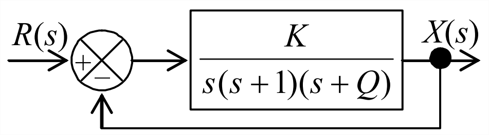
   Figure \(\PageIndex{1}\) (Copyright; author via source)

3. Consider the characteristic equation \(p^{2}+2 C p+K=0\). With mass \(m\) being positive-definite, this is the characteristic equation of the standard mass-damper-spring system described by equation of motion \(m \ddot{x}+c \dot{x}+k x=f_{x}(t)\), but with the notation \(C \equiv c /(2 m)\) and \(K \equiv k / m\). The roots of this 2^nd degree polynomial equation are the poles of the system transfer function. Suppose that damping constant \(C=6\) sec^-1, and that you want to evaluate the system stability characteristics for different values of stiffness constant \(K\) sec^-2. Consider first non-negative values of \(K\). For what positive value of \(K \equiv K_{c}\) is the damping critical, and what values do the polynomial roots have for \(K \equiv K_{c}\)? (Definition: if damping is positive but less than critical, then the roots are complex, corresponding to initial-condition response that is oscillation modulated by a decaying exponential envelope; if, on the other hand, damping is equal to or greater than critical, then the roots are negative real, corresponding to monotonic exponentially decaying initial-condition response.) What values are the roots for \(K = 0\) and for \(K=2 K_{c}\)? Show each of these roots by marking large \(\times\)’s at the correct positions on a complex \(p\)-plane graph [\(x\)-axis is \(\operatorname{Re}(p)\), \(y\)-axis is \(\operatorname{Im}(p)\), both in sec^-1]; label the axes and the linear scale of the axes, the same scale on both axes, as on the MATLAB graph Figure 16.8. Explain concisely what quality of the roots indicates that the system is stable for all values of \(K>0\). Now calculate the values of the roots for a negative stiffness, say \(K=-3 K_{c}\), and mark those roots on your \(p\)-plane graph. From the roots for a negative stiffness, what can you state conclusively about the system stability for all negative values of \(K\)? Indicate clearly on your \(p\)-plane graph the loci of roots as K increases from \(-3 K_{c}\) to 0, then from 0 to \(+K_{c}\), then from \(K_{c}\) to \(2 K_{c}\), and finally for \(K_{c}>2 K_{c}\). Is there a break-away point on your loci of roots; if so, for what value of \(K\)?
4. The following characteristic equations are expressed in completely or partially factored forms. For whichever equations are assigned, find the order \(n\) of the associated system, solve for the roots and mark their locations with large \(\times\)’s on a sketch of the complex \(p\)-plane, and state whether the system is stable or unstable; give the reason(s) for your conclusion.
   1. \((p-4)(p+3)(p+4)(p+5)=0\)
   2. \(p(p+2)\left(p^{2}-6 p+34\right)=0\)
   3. \((p+1)(p+3-j 5)(p+3+j 5)=0\)
   4. \((p+3)\left(p^{2}+2 p+2\right)\left(p^{2}+4 p+20\right)=0\)
5. The Laplace block diagram at right represents a system similar to that of Figures 16.3.1 and 16.3.2: it is a damped rotor with position feedback that is low-pass-filtered. But the low-pass filter in this case is 2^nd order, whereas the filter of Figure 16.3.2 is 1^st order. The filter transfer function on the block diagram is from Equation 10.2.3: low-pass break frequency \(\omega_{b}\) is the undamped natural frequency, and \(\gamma\) is the filter viscous damping ratio. We specify the value \(\gamma=1 / \sqrt{2}\); as shown on the frequency-response magnitude-ratio graph of Figure 10.2.1, for this \(\gamma\), the magnitude attenuation at \(\omega=\omega_{b}\) is \(1 / \sqrt{2}\) (same as for a 1^st order filter), and the high frequency roll-off is two decades for each decade increase of frequency (twice as steep as the roll-off of a 1^st order filter). (See also the discussion of 2^nd order low-pass filters at the end of Section 10.2.)

   

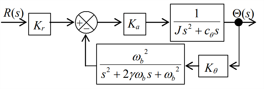
   Figure \(\PageIndex{2}\) (Copyright; author via source)

   1. Derive from the block diagram the algebraic equation for the closed-loop transfer function, \(\operatorname{CLTF}(s) \equiv \Theta(s) / R(s)\) (in terms of the symbols shown, without numbers at this stage). From your \(\operatorname{CLTF}(s)\), write the characteristic equation, \(\operatorname{Den}(p)=0\).
   2. Use the same values as for the calculations of Chapter 16: \(\omega_{b}=300\) rad/s and \(c_{\theta} / J=100\) s^-1, as well as \(\gamma=1 / \sqrt{2}\). Also as in Chapter 16, denote the varying control-system parameter as \(\Lambda \equiv K_{a} K_{\theta} / J\). Use MATLAB’s root operation to calculate, print out, and plot the loci of roots of this system over the entire range of \(\Lambda\) values for which the system is positively stable. Your graph and numerical output should show with at least 2-3 significant-figure precision any break-away points and the upper and lower boundaries of stability. Find by trial and error the approximate value of \(\Lambda\) for which the dominant oscillatory mode of response has the system damping ratio \(\zeta \approx 1 / \sqrt{2}\), and also calculate the time constant \(\tau_{2}\) and the frequency \(\omega_{d}\) for this value of \(\Lambda\).
6. The Laplace block diagram here represents a system to control the angular position of a satellite in one plane. The unfamiliar input-error block in the forward branch of the loop is the transfer function of a compensator, which in this case is designed to place a pair of the system’s closed-loop poles at \(2 \pi(-1 \pm j 1)\) s^-1 in the \(p\)-plane, for one value of control parameter \(\Lambda \equiv K_{c} K_{a} K_{\theta} / J\). For these poles, the frequency is \(f_{d}=\omega_{d} / 2 \pi=1\) Hz, and the viscous damping ratio is \(\zeta=1 / \sqrt{2}\).

   

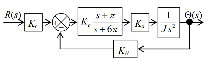
   Figure \(\PageIndex{3}\) (Copyright; author via source)

   1. Derive from the block diagram the algebraic equation for the closed-loop transfer function, \(\Theta(s) / R(s)\), then write the characteristic equation, \(\operatorname{Den}(p)=0\).
   2. Use MATLAB’s root operation to calculate, print out, and plot the loci of roots of this system over the parameter range \(0 \leq \Lambda \leq 200\) s^-2.
   3. Use Evans’ root-locus method to determine the numerical value of \(\Lambda\) that produces poles \(2 \pi(-1 \pm j 1)\) s^-1.
7. (Adapted from Franklin, et al., 1991, Problem 5.25 on page 347) The Laplace block diagram of the speed-control system of a magnetic-tape drive is shown in the figure below. The operator setting is input voltage signal \(e_{i n}(t)\), the Laplace transform of which is \(E_{i n}(s)\). Each major sub-system of the control system functions as a 1^st order system. The sub-system consisting of a power amplifier and a torque actuator has variable sensitivity \(K_{a}\) (N-m/V) and time constant \(\tau_{a}=1.0\) s. The tape drive has rotational inertia \(J = 4.0\) N-m per rad/s² and lubricated-shaft viscous damping constant \(c_{\theta}=1.0\) N-m per rad/s; the output of the tape drive in this application is rotational speed \(p(t)\) in rad/s [with Laplace transform \(P(s)\)], not rotational position \(\theta(t)\). The rotational-speed sensor in the feedback branch has sensitivity \(K_{p}\) = 1.250 V per rad/s; this sensor is sufficiently slow relative to the other sub-systems that we must account for its time constant, \(\tau_{p}=0.5\) s.
   1. Derive the closed-loop transfer function \(P(s) / E_{i n}(s)\), and then show that the characteristic equation of this system can be expressed as\[\left(p+c_{\theta} / J\right)\left(p+\tau_{a}^{-1}\right)\left(p+\tau_{p}^{-1}\right)+\Lambda=0, \text { or } r_{1} e^{j \theta_{1}} \times r_{2} e^{j \theta_{2}} \times r_{3} e^{j \theta_{3}}=\Lambda \exp [j(\pm \pi, \pm 3 \pi, \ldots)] \nonumber \]where the variable control parameter is defined as \(\Lambda=K_{a} K_{p} /\left(J \tau_{a} \tau_{p}\right)\), with units of s^-3.
   2. Determine (by hand, not MATLAB) all of the open-loop poles, all of the asymptotes (as \(\Lambda \rightarrow \infty\)) of the closed-loop poles, and the directions of departure of the root loci from the open-loop poles as \(\Lambda\) increases from zero. Sketch on graph paper a \(p\)-plane, and indicate on it the information that you determined for this system. See Figure 16.6.2 for an example of the type of diagram that yours should be. Make educated guesses and sketch on your diagram the forms you think the root loci should have.
   3. From part 16.7.1, any point on a locus of roots must satisfy the angle equality: \(\theta_{1}+\theta_{2}+ \theta_{3}=\pm \pi, \pm 3 \pi, \ldots\). Use this equality to write a transcendental equation that can be solved for the closed-loop pole \(j \omega_{d}\) at the upper stability boundary \(\Lambda_{u b}\) of the complex oscillatory loci; your equation will include trigonometric functions for the \(\theta_{i}\) angles that involve \(\omega_{d}\) and the numerical values of the open-loop poles. It is not necessary for you to solve the transcendental equation, but you may show just by substitution that \(\omega_{d}=1.6583124\) s^-1 \(=\sqrt{11} / 2\) s^-1 is the solution. Finally, again using the result of part 16.7.1, solve for the value \(\Lambda_{u b}=r_{1} \times r_{2} \times r_{3}\); your equation will include terms for the \(r_i\) magnitudes that involve \(\omega_{d}\) and the numerical values of the open-loop poles. [Note: you could also solve this part by applying Routh’s criteria, Equations 16.3.5 and 16.3.6, to calculate \(\Lambda_{u b}\), then substituting \(\Lambda_{u b}\) back into the characteristic equation to solve for \(p=j \omega_{d}\).]
8. The open-loop transfer function of a certain control system is\[G(s) H(s) \equiv O L T F(s)=\Lambda \frac{s^{2}+4 s+104}{(s+1)\left(s^{2}+2 s+26\right)} \nonumber \]where \(\Lambda\) (with units s^-1) is a variable parameter with possible range \(0 \leq \Lambda<+\infty\).
   1. Determine (by hand, not MATLAB) all of the open-loop poles and open-loop zeros of this system, any asymptotes (as \(\Lambda \rightarrow \infty\)) of the closed-loop poles, and the directions of departure of the root loci from the open-loop poles as \(\lambda\) increases from zero. Sketch on graph paper a \(p\)-plane, and indicate on it the information that you determine for this system. See Figure 16.6.2 for an example of the type of diagram that yours should be. However, whereas Figure 16.6.2 does not display any open-loop zeros, your diagram should; it is traditional to mark an open-loop zero by an \(\text {O}\), just as an open-loop pole is marked by an \(\times\). Make educated guesses and sketch on your diagram the forms you think the root loci should have.
   2. Show that the characteristic equation of the closed-loop system is\[p^{3}+(3+\Lambda) p^{2}+4(7+\Lambda) p+26(1+4 \Lambda)=0 \nonumber \]Apply Routh’s criteria, Equations 16.3.5 and 16.3.6, to calculate bounds and ranges of \(\Lambda\) for stability; in particular, solve a quadratic equation in unknown \(\Lambda\) to show that two of the bounds are \(\Lambda_{1,2}=8 \pm \sqrt{49.5}\) s^-1 = 0.964376 s^-1 and 15.0356 s^-1. In order to interpret the significance of these bounds relative to stability, calculate the quadratic equation for values of \(\Lambda\) slightly above and below these two bounds. Next, substitute the values \(\Lambda_1\) and \(\Lambda_2\) back into the characteristic equation as \(p=j \omega_{d 1}\) and \(p=j \omega_{d 2}\) to solve for the oscillatory frequencies \(\omega_{d 1}\) and \(\omega_{d 2}\) at \(\Lambda_1\) and (\Lambda_2\), respectively—there will be both a real and an imaginary part of the equation that you can solve; calculate the \(\omega_{d 1,2}\) from the easier part, then just substitute that value of \(\omega_{d 1,2}\) into the harder part to show that it also is satisfied. What is the significance of \(\omega_{d 1,2}\) and \(\Lambda_{1,2}\) on your diagram in part 16.8.1?
9. The characteristic equation of a certain LTI-SISO system can be expressed as\[1+G(p) H(p)=1+\Lambda \frac{p+1}{(p-1)(p+3)\left(p^{2}+2 p+2\right)}=0 \nonumber \]where \(\Lambda\) is a variable gain parameter with possible range \(0 \leq \Lambda<+\infty\).
   1. Determine (by hand, not MATLAB) all of the open-loop poles and the open-loop zero of this system, all of the asymptotes (as \(\Lambda \rightarrow \infty\)) of the closed-loop poles, and the directions of departure of the root loci from the open-loop poles as \(\Lambda\) increases from zero. Sketch on graph paper a \(p\)-plane, and indicate on it the information that you determine for this system. See Figure 16.6.2 for an example of the type of diagram that yours should be. However, whereas Figure 16.6.2 does not display any open-loop zeros, your diagram should; it is traditional to mark an open-loop zero by an \(\text{o}\), just as an open-loop pole is marked by an \(\times\). Make educated guesses and sketch on your diagram the forms you think the root loci should have.
   2. Your information in part 16.9.1 should suggest that one locus of roots is on the \(\operatorname{Re}(p)\) axis, starting from an open-loop pole at \(p=+1\) (for \(\Lambda=0\)), and terminating on an open-loop zero at \(p=-1\) (for \(\Lambda \rightarrow \infty\)). If that is true, then this particular locus must, for some value of \(\Lambda\) between 0 and \(\inf\), cross the origin of the \(p\)-plane from \(p > 0\) (unstable) to \(p < 0\) (stable). Your assignment is to express the characteristic equation in polar form [in the manner of Equations 16.5.4 - 16.5.7], use that form to prove the segment \(-1 \leq p \leq+1\) of the \(\operatorname{Re}(p)\) axis is or is not a locus, and, if it is, find the value of \(\Lambda\) at \(p = 0\), the boundary between instability and stability.
   3. Your solution from part 16.9.2 should indicate: there is a locus on the segment \(-1 \leq p \leq+1\) of the \(\operatorname{Re}(p)\) axis; and that locus has stable roots for \(\Lambda\) greater than its value at \(p = 0\). On the other hand, your information from part 16.9.1 should show there is a pair of complex conjugate open-loop poles in the stable western half-plane; it also should suggest that the loci departing from those complex open-loop poles (for \(\Lambda=0\)) then proceed in an easterly direction as \(\Lambda\) increases from zero, then, for some positive value of \(\Lambda\), cross over the \(\operatorname{Im}(p)\) axis into the unstable eastern half-plane. So, as \(\Lambda\) increases from zero, one real locus of closed-loop roots goes from being unstable to stable, but a pair of complex conjugate loci go from being stable to unstable. Therefore, we must ask if there is any range of \(\Lambda\) for which all of the loci are in the western half-plane and the closed-loop system is stable? Perhaps the best way to answer this question is to use Routh’s stability criteria. Consider a general 4^th order characteristic equation: \(a_{1} p^{4}+a_{2} p^{3}+a_{3} p^{2}+a_{4} p+a_{5}=0\). The associated system is stable if and only if all of the following conditions are satisfied (Ogata, 2001, pages 275-277):

      * all \(a_{i}>0, i=1,2,3,4,5\);

      * \(R_{2} \equiv a_{2} \times a_{3}-a_{1} \times a_{4}>0\);

      * \(R_{3} \equiv R_{2} \times a_{4}-a_{2}^{2} \times a_{5}>0\).

      Use Routh’s stability criteria to determine the range of \(\Lambda\) for which the closed-loop system is stable, if there is such a range.

10. (adapted from Nelson, 1989, Problem 7.7 on pages 222-223) The 1903 Wright Flyer by itself was inherently unstable in longitudinal motion (coupled pitch and vertical translation). However, Wilbur and Orville Wright stabilized, just barely, the system of airplane + pilot by providing sufficient control authority with a canard and by developing flying skill through extensive experimentation and practice with piloted gliders. A mathematical model¹ of the system was formulated, the Laplace block diagram for which is shown below. The input to the system is commanded pitch attitude \(\theta_{c}(t)\), and the output is actual pitch attitude \(\theta(t)\). Incremental canard position is \(\delta(t)\), for which the Laplace transform is \(\Delta(s)\). The canard-position-to-pitch-attitude transfer function incorporates both rigid-body dynamics and aerodynamics; the estimated model of this transfer function is\[\frac{\Theta(s)}{\Delta(s)}=\frac{11.0(s+0.5)(s+3.0)}{\left(s^{2}+5.9 s-11.9\right)\left(s^{2}+0.72 s+1.44\right)}=\frac{11.0(s+0.5)(s+3.0)}{(s-1.589)(s+7.489)\left(s^{2}+0.72 s+1.44\right)} \nonumber \]

    

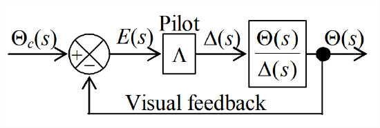
    Figure \(\PageIndex{4}\) (Copyright; author via source)

    1. Determine (by hand, not MATLAB) all of the open-loop poles and open-loop zeros of this system, all of the asymptotes (as pilot gain \(\Lambda \rightarrow \infty\)) of the closed-loop poles, and the directions of departure of the root loci from the open-loop poles as \(\Lambda\) increases from zero. Sketch on graph paper a \(p\)-plane, and indicate on it the information that you determined for this system. See Figure 16.6.2 for an example of the type of diagram that yours should be. However, whereas Figure 16.6.2 does not display any open-loop zeros, your diagram should; it is traditional to mark an open-loop zero by an \(\text{o}\), just as an open-loop pole is marked by an \(\times\).
    2. Show in detail that the characteristic polynomial equation in the form \(a_{1} p^{4}+a_{2} p^{3}+ a_{3} p^{2}+a_{4} p+a_{5}=0\), with all \(a_i\) coefficients either numerical or combinations of numbers and pilot gain \(\Lambda\), is given by:\[p^{4}+6.62 p^{3}+(11 \Lambda-6.212) p^{2}+(38.5 \Lambda-0.072) p+(16.5 \Lambda-17.136)=0 \nonumber \]
    3. If we wish at this point to program into software the calculation of loci of roots, we know only to consider \(0<\Lambda<\infty\); but, without more information, it is difficult to know what specific range or even order of magnitude of \(\Lambda\) to enter initially in the calculations. However, Routh’s stability criteria can provide that necessary additional information. Use Routh’s criteria [homework Problem 16.9.3] and the characteristic-equation coefficients to evaluate the absolute stability of the Wright Flyer system, thereby determining quantitatively a candidate range of \(\Lambda\) for use in calculation of loci of roots.² (Answer: for stability, \(\Lambda > 1.3096\))
    4. Use MATLAB’s root operation to calculate, print out, and plot the loci of roots of this system over a range of \(\Lambda\) values for which the system is stable. From Equation 9.5.5, viscous damping ratio \(\zeta=0.11\) of the oscillatory mode produces 50% amplitude decay during each cycle; show from your calculations that \(\Lambda=3.24\) is the lower pilot gain for which \(\zeta=0.11\), to reasonable engineering accuracy. From your results for \(\Lambda=3.24\), do you expect an oscillatory mode to be dominant in time response, or an exponential mode, or perhaps a combination of the two?
    5. It is of interest to examine in more detail the case of pilot gain \(\Lambda=3.24\), beginning with the closed-loop transfer function \(C L T F(s)\). Note that we essentially already have the denominator of \(C L T F(s)\): in the characteristic equation of part 16.10.2, just replace \(p \rightarrow s\) and set \(\Lambda=3.24\). Show that the closed-loop transfer function, in the form of Equation 16.1.6, is:\[C L T F(s)=\frac{\Theta(s)}{\Theta_{c}(s)}=\frac{35.64\left(s^{2}+3.5 s+1.5\right)}{s^{4}+6.62 s^{3}+29.428 s^{2}+124.668 s+36.324} \nonumber \]Now apply MATLAB’s residue operation (see homework Problem 2.15) to calculate the residues and poles of \(C L T F(s)\), and write out the partial-fraction expansion form of \(C L T F(s)\). Note that the poles found in this step should match those of part 16.10.4 for \(\Lambda=3.24\).
    6. Finally, consider a forced-response solution in time, with zero initial conditions. Suppose the pilot commands a short pulse to the pitch-control lever; represent this pulse approximately with a Dirac delta function (Section 8.4): \(\theta_{c}(t)=I_{\theta} \delta(t)\), for which the Laplace transform is \(\Theta_{c}(s)=I_{\theta}\). Let the impulse magnitude be \(I_{\theta}=2\) degree-s. Use the partial-fraction expansion form of \(C L T F(s)\) from part 16.10.5 to derive the equation for the pitch response \(\theta(t)\) to this control excitation, and then calculate and plot this transient response over a 15-s interval.
11. We know from Chapter 16 that the process of calculating and plotting loci of roots is useful in analysis of control-system stability; the objective of this problem is to illustrate another important application of root-loci: analysis of the stability of a system for which the potentially destabilizing feedback is natural and intrinsic, not human-designed. Systems with this characteristic are often described as self-excited (see, e.g., Den Hartog, 1956, Chapter 7). The particular phenomenon we consider here, aeroelastic dynamic response of a typical-section airfoil, including unstable flutter, originated in aeronautical engineering but is relevant also to many other applications of force-generating objects that are immersed within moving fluids (e.g., hydrofoils, wind-turbine blades, and propellers). The typical-section airfoil is described in Section 11.3, Examples 11.3.2 and 11.3.3, and we consider here the form depicted below, an uncambered, symmetric thin airfoil supported by springs in a wind tunnel, and immersed within an incompressible airstream of density \(\rho\) and freestream velocity \(V\).

    

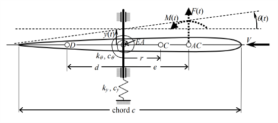
    Figure \(\PageIndex{5}\) (Copyright; author via source)

    Structural dynamic equations of motion with vertical translation of mass center \(C\), \(y_{A C}(t)\), and pitch \(\theta(t)\) as degrees of freedom (DOFs) are derived and expressed in matrix form in Equation 11.3.16. However, a more appropriate vertical translation DOF for this problem is \(y_{E A}(t) \equiv y(t)\) of the elastic axis \(EA\), as labeled on the figure above; the equations of motion for DOFs \(y(t)\) and \(\theta(t)\) are derived in homework Problem 11.4 and are expressed below, with the addition of a damping matrix that represents approximately the energy dissipation within the springs (using the viscous-damping mathematical model described in Appendix B, Section 19.5).\[\left[\begin{array}{cc}
    m & m r \\
    m r & J_{E A}
    \end{array}\right]\left[\begin{array}{l}
    \ddot{y} \\
    \ddot{\theta}
    \end{array}\right]+\left[\begin{array}{cc}
    c_{y} & 0 \\
    0 & c_{\theta}
    \end{array}\right]\left[\begin{array}{l}
    \dot{y} \\
    \dot{\theta}
    \end{array}\right]+\left[\begin{array}{cc}
    k_{y} & 0 \\
    0 & k_{\theta}
    \end{array}\right]\left[\begin{array}{l}
    y \\
    \theta
    \end{array}\right]=\left[\begin{array}{c}
    F(t) \\
    M(t)+F(t) e
    \end{array}\right]\label{eqn:P16.11.1} \]We assume that aerodynamic resultant lift force and moment (positive nose-up) are due both to the motions of the typical section itself (self-excitation), and to sources such as gusts that are independent of the motion, which we denote as lift \(F_{G}(t)\) and moment \(MG(t)\). There is no exact and readily applicable theory of unsteady, motion-dependent aerodynamics; therefore, we use here one of the many approximate theories, the quasisteady aerodynamics of Fung, 1955, pages 191-193. In these equations of unsteady lift and moment, we replace Fung’s lift-curve slope for an airfoil of infinite span, \(C_{L \alpha}=2 \pi\) per radian, with a reduced value of \(C_{L \alpha}\) that applies for an airfoil of finite span. This is appropriate for the specific numerical parameters considered below in part 16.11.2, which are chosen to represent an actual experimental research investigation of typical-section aeroelasticity. Since dynamic pressure is \(\bar{q}=1 / 2 \rho V^{2}\), it is appropriate to define in Fung’s equations the constant \(K \equiv 1 / 2 \rho S(2 \pi) \rightarrow K \equiv 1 / 2 \rho S C_{L \alpha}\). Thus, the motion-dependent and motion-independent aerodynamic resultant lift and nose-up moment are written as:\[F(t)=\bar{q} S C_{L \alpha}\left(\theta-\frac{\dot{y}-d \dot{\theta}}{V}\right)+F_{G}(t)=K\left(V^{2} \theta-V \dot{y}+d V \dot{\theta}\right)+F_{G}(t)\label{eqn:P16.11.2a} \]\[M(t)=-\bar{q} S c \frac{\pi c}{8} \frac{\dot{\theta}}{V}+M_{G}(t)=-K \frac{\pi / 8}{C_{L \alpha}} c^{2} V \dot{\theta}+M_{G}(t)\label{eqn:P16.11.2b} \]

    1. Substitute Equations \(\ref{eqn:P16.11.2a}\) and \(\ref{eqn:P16.11.2b}\) into Equation \(\ref{eqn:P16.11.1}\), then transpose the motion-dependent terms from the right-hand side to the left-hand side so that the damping and stiffness matrices in Equation \(\ref{eqn:P16.11.1}\) become more general; for example, the structural-plus-aerodynamic stiffness matrix becomes \(\left[\begin{array}{cc}
       k_{y} & -K V^{2} \\
       0 & k_{\theta}-e K V^{2}
       \end{array}\right]\). Now you have a set of equations that, in principle, can be solved for DOFs \(y(t)\) and \(\theta(t)\) by Laplace transformation. Assume null initial conditions, \(y(0)=0\) and \(\theta(0)=0\), and assume that \(F_{G}(t)\) and \(M_{G}(t)\) are Laplace transformable functions, then express the Laplace-transformed equations of motion in the following form, writing explicit quadratic (in \(s\)) polynomials for the four \(M_{i j}(s ; V)\) elements of the left-hand side coefficient matrix:\[\left[\begin{array}{ll}
       M_{11}(s ; V) & M_{12}(s ; V) \\
       M_{21}(s ; V) & M_{22}(s ; V)
       \end{array}\right]\left[\begin{array}{l}
       Y(s) \\
       \Theta(s)
       \end{array}\right] \equiv[\mathbf{M}(s ; V)]\left[\begin{array}{c}
       Y(s) \\
       \Theta(s)
       \end{array}\right]=\left[\begin{array}{c}
       L\left[F_{G}(t)\right] \\
       L\left[M_{G}(t)\right]+e L\left[F_{G}(t)\right]
       \end{array}\right]\label{eqn:P16.11.3} \]The matrix solution of Equation \(\ref{eqn:eqn:P16.11.3}\) can be written as\[\left[\begin{array}{c}
       Y(s) \\
       \Theta(s)
       \end{array}\right]=[\mathbf{T} \mathbf{F}(s ; V)]\left[\begin{array}{c}
       L\left[F_{G}(t)\right] \\
       L\left[M_{G}(t)\right]+e L\left[F_{G}(t)\right]
       \end{array}\right]\label{eqn:P16.11.4} \]where the \(2 \times 2\) coefficient matrix \([\mathrm{TF}(s ; V)]=[\mathbf{M}(s ; V)]^{-1}\) is the multiple-input-multiple-output (MIMO) transfer-function matrix relating two outputs, \(Y(s)\) and \(\Theta(s)\), to two inputs, \(L\left[F_{G}(t)\right]\) and \(\left(L\left[M_{G}(t)\right]+e L\left[F_{G}(t)\right]\right)\); however, it is clear that each element of matrix \([\mathbf{T F}(s ; V)]\) is itself a single-input-single-output (SISO) transfer function. Use Equations 12.2.16-12.2.18 to write an equation for \([\mathbf{T F}(s ; V)]\) in terms of the four \(M_{i j}(s ; V)\) elements. Note, in particular, that the denominator of each of the SISO transfer functions, \(T F_{i j}(s ; V)\), is the determinant \(\operatorname{det}[\mathbf{M}(s ; V)]=M_{11}(s ; V) \times M_{22}(s ; V)-M_{21}(s ; V) \times M_{12}(s ; V)\). By the logic of Section 16.1, therefore, the quartic (in \(p\)) polynomial equation, \(\operatorname{det}[\mathbf{M}(p ; V)]=0\), is the general characteristic equation of the system, and its four roots \(p_{i}(V)\) at each freestream airspeed \(V\) determine both the character of unforced time response (e.g., exponential, oscillatory, etc.) and the system stability or instability at that particular airspeed.
    2. In this part, you will use the equations of part 16.11.1 to calculate and plot the loci of roots, as wind-tunnel freestream airspeed \(V\) varies, using numerical parameters that were selected to represent the research project of a Brazilian group, DeMarqui, et al., 2005 and 2006. The parameters of the typical-section airfoil and the wind-tunnel atmosphere are:

       Mass \(m\) = 18.0 kg

       Rotational inertia about mass center \(C\): \(J_C\) = 0.219 kg-m²; so \(J_{E A}=J_{C}+m r^{2}\)

       Offset of mass center \(C\) forward of elastic axis \(EA\): \(r\) = 5 mm = 0.005 m

       Stiffness constant of vertical-translation spring: \(k_y\) = 1,110 N/m

       Stiffness constant of pitch-rotation spring: \(k_\theta\) = 49.8 N-m/radian

       Viscous-damping constant of vertical-translation spring: \(c_{\theta}=0.00318\) s \(\times k_{y}\)

       Viscous-damping constant of pitch-rotation spring: \(c_{\theta}=0.00318\) s \(\times k_{\theta}\)

       Planform: chord \(c\) = 0.45 m; span = 0.80 m; so, area \(S=c \times\) span = 0.36 m²

       Offset of \(\frac{1}{4}\)-chord aerodynamic center \(AC\) forward of elastic axis \(E A: d=c / 4\)

       Offset of \(\frac{3}{4}\)-chord dynamic-pitch point \(D\) aft of elastic axis \(E A: d=c / 4\)

       Standard air density at 800-m average altitude of Sao Paulo, Brazil: \(\rho=1.1337\) kg/m³

       Lift-curve slope for this low-aspect-ratio airfoil: \(C_{L \alpha}=2.64\) per radian

       The most significant single result that you seek is the wind-tunnel freestream airspeed \(V_F\) at which the typical section experiences aeroelastic flutter. The flutter airspeed \(V_F\) is that value of \(V\) at which the dominant time response of the typical section is a pure sinusoid; for lower airspeeds, \(0 \leq V<V_{F}\), the dominant response is stable positively damped oscillation; but for higher airspeeds, \(V>V_{F}\), the dominant response is unstable exponentially expanding oscillation. Begin the numerical analysis by using Equation 11.3.10 to calculate the aeroelastic divergence airspeed \(V_{D}\) in m/s; because usually \(V_{D}>V_{F}\), this value of \(V_{D}\) will suggest to you the range of airspeeds, \(0 \leq V<V_{D}\), over which you should calculate the loci of roots in order to determine \(V_{F}\). Use MATLAB’s conv and root operations to calculate, print out, and plot the loci of roots of characteristic equation \(M_{11}(p ; V) \times M_{22}(p ; V)-M_{21}(p ; V) \times M_{12}(p ; V)=0\). You might find useful the form of MATLAB script M-file MATLABdemo164.m that produced Figures 16.5.1 and 16.5.5 in Section 16.5. In this problem, freestream velocity \(V\) plays the same role that control gain parameter \(\Lambda\) plays in MATLABdemo164.m.

¹Culick, F.E.C.: “Building a 1903 Wright ‘Flyer’—by Committee,” AIAA Paper 88-0094, 1988

²This exercise requires several calculations. Rather than calculating manually, you might prefer to use symbolic software. If you use MATLAB’s Symbolic Math Toolbox (see homework Problem 1.6), be aware that this symbolic software performs calculations exactly, expressing numbers as fractions of integers if at all possible. But the integers in these fractions can become quite large and unwieldy. You can convert these fractions into decimal numbers by using “variable precision arithmetic.” For example, if a symbolic term is expressed as v = 4115/2263*w, you can convert the fractional coefficient into a five-digit decimal with the operations >> digits(5);v5=vpa(v), the result of which is v5 = 1.8184*w.