
1.3: Signal Operations
- Page ID
- 22839

Introduction
This module will look at two signal operations affecting the time parameter of the signal, time shifting and time scaling. These operations are very common components to real-world systems and, as such, should be understood thoroughly when learning about signals and systems.
Manipulating the Time Parameter
Time Shifting
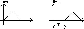
Time shifting is, as the name suggests, the shifting of a signal in time. This is done by adding or subtracting a quantity of the shift to the time variable in the function. Subtracting a fixed positive quantity from the time variable will shift the signal to the right (delay) by the subtracted quantity, while adding a fixed positive amount to the time variable will shift the signal to the left (advance) by the added quantity.
Time Scaling
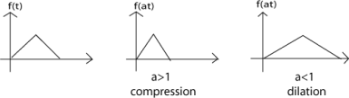
Time scaling compresses or dilates a signal by multiplying the time variable by some quantity. If that quantity is greater than one, the signal becomes narrower and the operation is called compression, while if the quantity is less than one, the signal becomes wider and is called dilation.
Example \(\PageIndex{1}\)
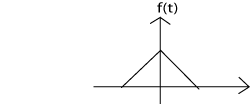
Given \(f(t)\) we would like to plot \(f(at−b)\).
Solution
The figure below describes a method to accomplish this.
 (a)
(a)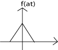 (b)
(b)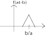 (c)
(c)
Figure \(\PageIndex{3}\): (a) Begin with \(f(t)\) (b) Then replace \(t\) with \(at\) to get \(f(at)\) (c) Finally, replace \(t\) with \(t−\frac{b}{a}\) to get \(f(a(t−\frac{b}{a}))=f(at−b)\)
Time Reversal
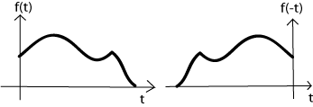
A natural question to consider when learning about time scaling is: What happens when the time variable is multiplied by a negative number? The answer to this is time reversal. This operation is the reversal of the time axis, or flipping the signal over the y-axis.
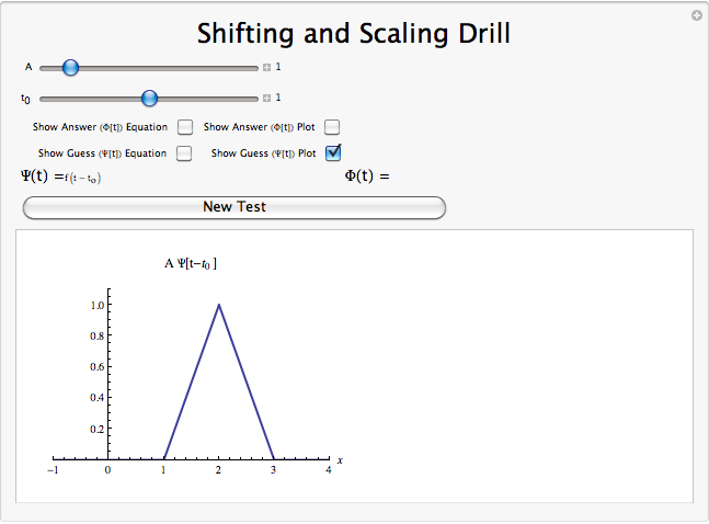
Time Scaling and Shifting Demonstration
Signal Operations Summary
Some common operations on signals affect the time parameter of the signal. One of these is time shifting in which a quantity is added to the time parameter in order to advance or delay the signal. Another is the time scaling in which the time parameter is multiplied by a quantity in order to dilate or compress the signal in time. In the event that the quantity involved in the latter operation is negative, time reversal occurs.