10.3: Signal Reconstruction

Introduction

The sampling process produces a discrete time signal from a continuous time signal by examining the value of the continuous time signal at equally spaced points in time. Reconstruction, also known as interpolation, attempts to perform an opposite process that produces a continuous time signal coinciding with the points of the discrete time signal. Because the sampling process for general sets of signals is not invertible, there are numerous possible reconstructions from a given discrete time signal, each of which would sample to that signal at the appropriate sampling rate. This module will introduce some of these reconstruction schemes.

Reconstruction

Reconstruction Process

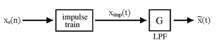
The process of reconstruction, also commonly known as interpolation, produces a continuous time signal that would sample to a given discrete time signal at a specific sampling rate. Reconstruction can be mathematically understood by first generating a continuous time impulse train

\[x_{i m p}(t)=\sum_{n=-\infty}^{\infty} x_{s}(n) \delta\left(t-n T_{s}\right) \nonumber \]

from the sampled signal \(x_s\) with sampling period \(T_s\) and then applying a lowpass filter \(G\) that satisfies certain conditions to produce an output signal \(\tilde{x}\). If \(G\) has impulse response \(g\), then the result of the reconstruction process, illustrated in Figure \(\PageIndex{1}\), is given by the following computation, the final equation of which is used to perform reconstruction in practice.

\[\begin{align}
\widetilde{x}(t) &=\left(x_{i m p} * g\right)(t) \nonumber \\
&=\int_{-\infty}^{\infty} x_{i m p}(\tau) g(t-\tau) d \tau \nonumber \\
&=\int_{-\infty}^{\infty} \sum_{n=-\infty}^{\infty} x_{s}(n) \delta\left(\tau-n T_{s}\right) g(t-\tau) d \tau \nonumber \\
&=\sum_{n=-\infty}^{\infty} x_{s}(n) \int_{-\infty}^{\infty} \delta\left(\tau-n T_{s}\right) g(t-\tau) d \tau \nonumber \\
&=\sum_{n=-\infty}^{\infty} x_{s}(n) g\left(t-n T_{s}\right)
\end{align} \nonumber \]

Figure \(\PageIndex{1}\): Block diagram of reconstruction process for a given lowpass filter \(G\).

Reconstruction Filters

In order to guarantee that the reconstructed signal \(\tilde{x}\) samples to the discrete time signal \(x_s\) from which it was reconstructed using the sampling period \(T_s\), the lowpass filter \(G\) must satisfy certain conditions. These can be expressed well in the time domain in terms of a condition on the impulse response \(g\) of the lowpass filter \(G\). The sufficient condition to be a reconstruction filters that we will require is that, for all \(n \in \mathbb{Z}\),

\[g\left(n T_{s}\right)=\left\{\begin{array}{ll}
1 & n=0 \\
0 & n \neq 0
\end{array}=\delta(n)\right. . \nonumber \]

This means that gg sampled at a rate \(T_s\) produces a discrete time unit impulse signal. Therefore, it follows that sampling \(\tilde{x}\) with sampling period \(T_s\) results in

\[\begin{align}
\widetilde{x}\left(n T_{s}\right) &=\sum_{m=-\infty}^{\infty} x_{s}(m) g\left(n T_{s}-m T_{s}\right) \nonumber \\
&=\sum_{m=-\infty}^{\infty} x_{s}(m) g\left((n-m) T_{s}\right) \nonumber \\
&=\sum_{m=-\infty}^{\infty} x_{s}(m) \delta(n-m) \nonumber \\
&=x_{s}(n),
\end{align} \nonumber \]

which is the desired result for reconstruction filters.

Cardinal Basis Splines

Since there are many continuous time signals that sample to a given discrete time signal, additional constraints are required in order to identify a particular one of these. For instance, we might require our reconstruction to yield a spline of a certain degree, which is a signal described in piecewise parts by polynomials not exceeding that degree. Additionally, we might want to guarantee that the function and a certain number of its derivatives are continuous.

This may be accomplished by restricting the result to the span of sets of certain splines, called basis splines or B-splines. Specifically, if a \(n\)th degree spline with continuous derivatives up to at least order \(n−1\) is required, then the desired function for a given \(T_s\) belongs to the span of \(\left\{B_{n}\left(t / T_{s}-k\right) \: | \: k \in \mathbb{Z}\right\}\) where

\[B_{n}=B_{0} * B_{n-1} \nonumber \]

for \(n≥1\) and

\[B_{0}(t)=\left\{\begin{array}{cc}
1 & -1 / 2<t<1 / 2 \\
0 & \text { otherwise }
\end{array}\right. . \nonumber \]

Figure \(\PageIndex{2}\): The basis splines \(B_n\) are shown in the above plots. Note that, except for the order 0 and order 1 functions, these functions do not satisfy the conditions to be reconstruction filters. Also notice that as the order increases, the functions approach the Gaussian function, which is exactly \(B_{\infty}\).

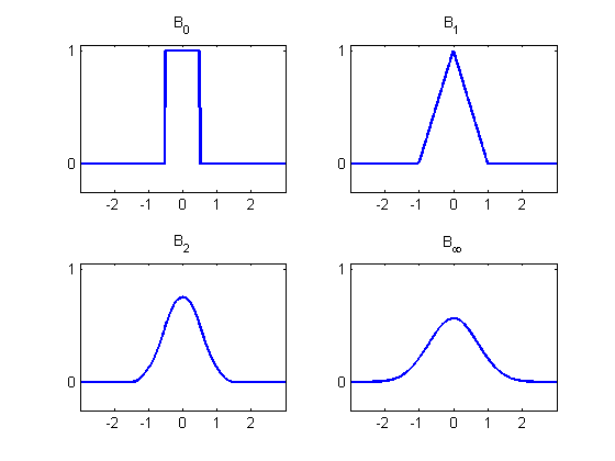
However, the basis splines \(B_n\) do not satisfy the conditions to be a reconstruction filter for \(n≥2\) as is shown in Figure \(\PageIndex{2}\). Still, the \(B_n\) are useful in defining the cardinal basis splines, which do satisfy the conditions to be reconstruction filters. If we let \(b_n\) be the samples of \(B_n\) on the integers, it turns out that \(b_n\) has an inverse \(b^{−1}_n\) with respect to the operation of convolution for each \(n\). This is to say that \(b_{n}^{-1} * b_{n}=\delta\). The cardinal basis spline of order nn for reconstruction with sampling period \(T_s\) is defined as

\[\eta_{n}(t)=\sum_{k=-\infty}^{\infty} b_{n}^{-1}(k) B_{n}\left(t / T_{s}-k\right). \nonumber \]

In order to confirm that this satisfies the condition to be a reconstruction filter, note that

\[\eta_{n}\left(m T_{s}\right)=\sum_{k=-\infty}^{\infty} b_{n}^{-1}(k) B_{n}(m-k)=\left(b_{n}^{-1} * b_{n}\right)(m)=\delta(m). \nonumber \]

Thus, \(\eta_n\) is a valid reconstruction filter. Since \(\eta_n\) is an \(n\)th degree spline with continuous derivatives up to order \(n−1\), the result of the reconstruction will be a \(n\)th degree spline with continuous derivatives up to order \(n−1\).

Figure \(\PageIndex{3}\): The above plots show cardinal basis spline functions \(\eta_0\), \(\eta_1\), \(\eta_2\), and \(\eta_{\infty}\). Note that the functions satisfy the conditions to be reconstruction filters. Also, notice that as the order increases, the cardinal basis splines approximate the sinc function, which is exactly \(\eta_{\infty}\). Additionally, these filters are acausal.

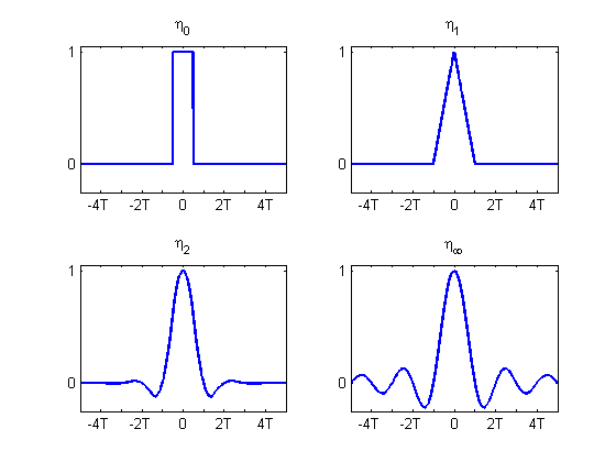
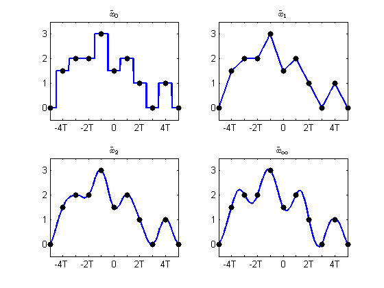
The lowpass filter with impulse response equal to the cardinal basis spline \(\eta_0\) of order 0 is one of the simplest examples of a reconstruction filter. It simply extends the value of the discrete time signal for half the sampling period to each side of every sample, producing a piecewise constant reconstruction. Thus, the result is discontinuous for all nonconstant discrete time signals.

Likewise, the lowpass filter with impulse response equal to the cardinal basis spline \(\eta_1\) of order 1 is another of the simplest examples of a reconstruction filter. It simply joins the adjacent samples with a straight line, producing a piecewise linear reconstruction. In this way, the reconstruction is continuous for all possible discrete time signals. However, unless the samples are collinear, the result has discontinuous first derivatives.

In general, similar statements can be made for lowpass filters with impulse responses equal to cardinal basis splines of any order. Using the \(n\)th order cardinal basis spline \(\eta_n\), the result is a piecewise degree nn polynomial. Furthermore, it has continuous derivatives up to at least order \(n−1\). However, unless all samples are points on a polynomial of degree at most \(n\), the derivative of order nn will be discontinuous.

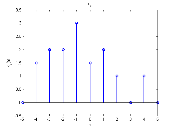
Reconstructions of the discrete time signal given in Figure \(\PageIndex{4}\) using several of these filters are shown in Figure \(\PageIndex{5}\). As the order of the cardinal basis spline increases, notice that the reconstruction approaches that of the infinite order cardinal spline \(\eta_{\infty}\), the sinc function. As will be shown in the subsequent section on perfect reconstruction, the filters with impulse response equal to the sinc function play an especially important role in signal processing.

Figure \(\PageIndex{4}\): The above plot shows an example discrete time function. This discrete time function will be reconstructed using sampling period \(T_s\) using several cardinal basis splines in Figure \(\PageIndex{5}\).

Figure \(\PageIndex{5}\): The above plots show interpolations of the discrete time signal given in Figure \(\PageIndex{4}\) using lowpass filters with impulse responses given by the cardinal basis splines shown in Figure \(\PageIndex{3}\). Notice that the interpolations become increasingly smooth and approach the sinc interpolation as the order increases.

Reconstruction Summary

Reconstruction of a continuous time signal from a discrete time signal can be accomplished through several schemes. However, it is important to note that reconstruction is not the inverse of sampling and only produces one possible continuous time signal that samples to a given discrete time signal. As is covered in the subsequent module, perfect reconstruction of a bandlimited continuous time signal from its sampled version is possible using the Whittaker-Shannon reconstruction formula, which makes use of the ideal lowpass filter and its sinc function impulse response, if the sampling rate is sufficiently high.