12.1: Z-Transform

Introduction

The Z transform is a generalization of the Discrete-Time Fourier Transform (Section 9.2). It is used because the DTFT does not converge/exist for many important signals, and yet does for the z-transform. It is also used because it is notationally cleaner than the DTFT. In contrast to the DTFT, instead of using complex exponentials (Section 7.2) of the form (e^{j \omega n}\), with purely imaginary parameters, the Z transform uses the more general, \(z^n\), where \(z\) is complex. The Z-transform thus allows one to bring in the power of complex variable theory into Digital Signal Processing.

The Z-Transform

Bilateral Z-transform Pair

Although Z transforms are rarely solved in practice using integration (tables and computers (e.g. Matlab) are much more common), we will provide the bilateral Z transform pair here for purposes of discussion and derivation. These define the forward and inverse Z transformations. Notice the similarities between the forward and inverse transforms. This will give rise to many of the same symmetries found in Fourier analysis (Section 5.1).

Z Transform

\[X(z)=\sum_{n=-\infty}^{\infty} x[n] z^{-n} \nonumber \]

Inverse Z Transform

\[x[n]=\frac{1}{2 \pi j} \oint_{r} X(z) z^{n-1} \mathrm{d} z \nonumber \]

Note

We have defined the bilateral z-transform. There is also a unilateral z-transform ,

\[X(z)=\sum_{n=0}^{\infty} x[n] z^{-n} \nonumber \]

which is useful for solving the difference equations with nonzero initial conditions. This is similar to the unilateral Laplace Transform in continuous time.

Relation between Z-transform and DTFT

Taking a look at the equations describing the Z-Transform and the Discrete-Time Fourier Transform:

Discrete-Time Fourier Transform

\[X\left(e^{j \omega}\right)=\sum_{n=-\infty}^{\infty} x(n) e^{-(j \omega n)} \nonumber \]

Z-Transform

\[X(z)=\sum_{n=-\infty}^{\infty} x[n] z^{-n} \nonumber \]

We can see many similarities; first, that:

\[X\left(e^{j \omega}\right)=X(z) \nonumber \]

for all \(z=e^{j \omega}\)

Visualizing the Z-transform

With the DTFT, we have a complex-valued function of a real-valued variable \(\omega\) (and \(2\pi\) periodic). The Z-transform is a complex-valued function of a complex valued variable z.

Plots

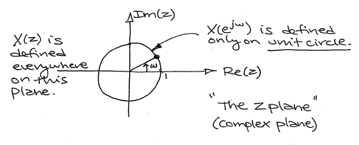
Figure \(\PageIndex{1}\)

With the Fourier transform, we had a complex-valued function of a purely imaginary variable, \(F(j \omega)\). This was something we could envision with two 2-dimensional plots (real and imaginary parts or magnitude and phase). However, with Z, we have a complex-valued function of a complex variable. In order to examine the magnitude and phase or real and imaginary parts of this function, we must examine 3-dimensional surface plots of each component.

Consider the z-transform given by \(H(z)=z\), as illustrated below.

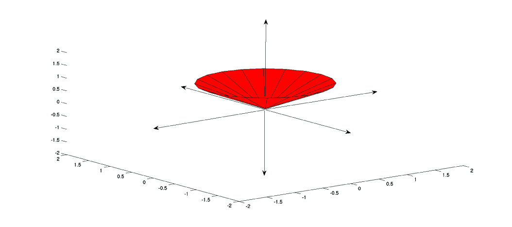
Figure \(\PageIndex{2}\)

The corresponding DTFT has magnitude and phase given below.

Note

While these are legitimate ways of looking at a signal in the Z domain, it is quite difficult to draw and/or analyze. For this reason, a simpler method has been developed. Although it will not be discussed in detail here, the method of Poles and Zeros is much easier to understand and is the way both the Z transform and its continuous-time counterpart the Laplace-transform are represented graphically.

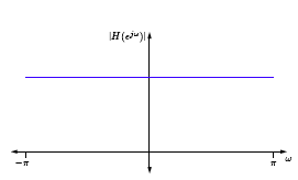
(a)

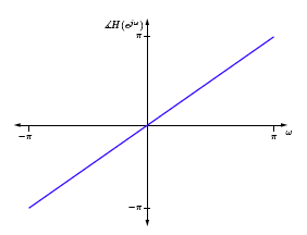
(b)

Figure \(\PageIndex{3}\): Magnitude and Phase of \(H(z)\).

What could the system H be doing? It is a perfect all-pass, linear-phase system. But what does this mean?

Suppose \(h[n]=\delta\left[n-n_{0}\right]\). Then

\[\begin{aligned}
H(z) &=\sum_{n=-\infty}^{\infty} h[n] z^{-n} \\
&=\sum_{n=-\infty}^{\infty} \delta\left[n-n_{0}\right] z^{-n} \\
&=z^{-n_{0}}
\end{aligned} \nonumber \]

Thus, \(H(z)=z^{−n_0}\) is the \(z\)-transform of a system that simply delays the input by \(n_0\). \(H(z)\) is the \(z\)-transform of a unit-delay.

Now consider \(x[n]=\alpha^{n} u[n]\)

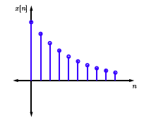
Figure \(\PageIndex{4}\)

\[\begin{align}
X(z) &=\sum_{n=-\infty}^{\infty} x[n] z^{-n}=\sum_{n=0}^{\infty} \alpha^{n} z^{-n} \nonumber \\
&=\sum_{n=0}^{\infty}\left(\frac{\alpha}{z}\right)^{n} \nonumber \\
&=\frac{1}{1-\frac{\alpha}{z}}\left( \text{ if }\left|\frac{\alpha}{z}\right|<1\right)(\text { Geometric series }) \nonumber \\
&=\frac{z}{z-\alpha}
\end{align} \nonumber \]

What if \(|\frac{\alpha}{z}|≥1\)? Then \(\sum_{n=0}^{\infty}\left(\frac{\alpha}{z}\right)^{n}\) does not converge! Therefore, whenever we compute a \(z\)-tranform, we must also specify the set of \(z\)'s for which the \(z\)-transform exists. This is called the region of convergence (ROC).

Note: Using a computer to find the Z-transform

Matlab has two functions,

ztrans

and

iztrans

that are both part of the symbolic toolbox, and will find the Z and inverse Z transforms respectively. This method is generally preferred for more complicated functions. Simpler and more contrived functions are usually found easily enough by using tables.

Application to Discrete Time Filters

The \(z\)-transform might seem slightly ugly. We have to worry about the region of convergence, and stability issues, and so forth. However, in the end it is worthwhile because it proves extremely useful in analyzing digital filters with feedback. For example, consider the system illustrated below

Plots

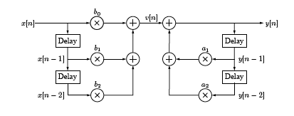
Figure \(\PageIndex{5}\)

We can analyze this system via the equations

\[v[n]=b_{0} x[n]+b_{1} x[n-1]+b_{2} x[n-2] \nonumber \]

and

\[y[n]=v[n]+a_{1} y[n-1]+a_{2} y[n-2] \nonumber \]

More generally,

\[v[n]=\sum_{k=0}^{N} b_{k} x[n-k] \nonumber \]

and

\[y[n]=\sum_{k=1}^{M} a_{k} y[n-k]+v[n] \nonumber \]

or equivalently,

\[\sum_{k=0}^{N} b_{k} x[n-k]=y[n]-\sum_{k=1}^{M} a_{k} y[n-k]. \nonumber \]

What does the \(z\)-transform of this relationship look like?

\[Z \sum_{k=0}^{M} a_{k} y[n-k]=Z \sum_{k=0}^{M} b_{k} x[n-k] \nonumber \]

\[\sum_{k=0}^{M} a_{k} Z\{y[n-k]\}=\sum_{k=0}^{M} b_{k} Z\{x[n-k]\} \nonumber \]

Note that

\[\begin{aligned}
Z\{y[n-k]\} &=\sum_{n=-\infty}^{\infty} y[n-k] z^{-n} \\
&=\sum_{m=-\infty}^{\infty} y[m] z^{-m} z^{-k} \\
&=Y(z) z^{-k}
\end{aligned} \nonumber \]

Thus the relationship reduces to

\begin{aligned}
\sum_{k=0}^{M} a_{k} Y(z) z^{-k} &=\sum_{k=0}^{N} b_{k} X(z) z^{-k} \\
Y(z) \sum_{k=0}^{M} a_{k} z^{-k} &=X(z) \sum_{k=0}^{N} b_{k} z^{-k} \\
\frac{Y(z)}{X(z)} &=\frac{\sum_{k=0}^{N} b_{k} z^{-k}}{\sum_{k=0}^{M} a_{k} z^{-k}}
\end{aligned}

Hence, given a system the one above, we can easily determine the system's transfer function, and end up with a ratio of two polynomials in \(z\): a rational function. Similarly, given a rational function, it is easy to realize this function in a simple hardware architecture.

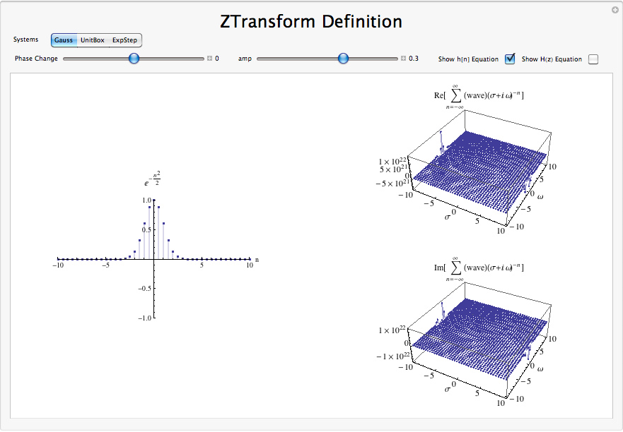
Interactive Z-Transform Demonstration

Figure \(\PageIndex{6}\): Interact (when online) with a Mathematica CDF demonstrating the Z Transform. To Download, right-click and save target as .cdf.

Conclusion

The z-transform proves a useful, more general form of the Discrete Time Fourier Transform. It applies equally well to describing systems as well as signals using the eigenfunction method, and proves extremely useful in digital filter design.