14.5: Eigenfunctions of LTI Systems
- Page ID
- 22932
\( \newcommand{\vecs}[1]{\overset { \scriptstyle \rightharpoonup} {\mathbf{#1}} } \)
\( \newcommand{\vecd}[1]{\overset{-\!-\!\rightharpoonup}{\vphantom{a}\smash {#1}}} \)
\( \newcommand{\id}{\mathrm{id}}\) \( \newcommand{\Span}{\mathrm{span}}\)
( \newcommand{\kernel}{\mathrm{null}\,}\) \( \newcommand{\range}{\mathrm{range}\,}\)
\( \newcommand{\RealPart}{\mathrm{Re}}\) \( \newcommand{\ImaginaryPart}{\mathrm{Im}}\)
\( \newcommand{\Argument}{\mathrm{Arg}}\) \( \newcommand{\norm}[1]{\| #1 \|}\)
\( \newcommand{\inner}[2]{\langle #1, #2 \rangle}\)
\( \newcommand{\Span}{\mathrm{span}}\)
\( \newcommand{\id}{\mathrm{id}}\)
\( \newcommand{\Span}{\mathrm{span}}\)
\( \newcommand{\kernel}{\mathrm{null}\,}\)
\( \newcommand{\range}{\mathrm{range}\,}\)
\( \newcommand{\RealPart}{\mathrm{Re}}\)
\( \newcommand{\ImaginaryPart}{\mathrm{Im}}\)
\( \newcommand{\Argument}{\mathrm{Arg}}\)
\( \newcommand{\norm}[1]{\| #1 \|}\)
\( \newcommand{\inner}[2]{\langle #1, #2 \rangle}\)
\( \newcommand{\Span}{\mathrm{span}}\) \( \newcommand{\AA}{\unicode[.8,0]{x212B}}\)
\( \newcommand{\vectorA}[1]{\vec{#1}} % arrow\)
\( \newcommand{\vectorAt}[1]{\vec{\text{#1}}} % arrow\)
\( \newcommand{\vectorB}[1]{\overset { \scriptstyle \rightharpoonup} {\mathbf{#1}} } \)
\( \newcommand{\vectorC}[1]{\textbf{#1}} \)
\( \newcommand{\vectorD}[1]{\overrightarrow{#1}} \)
\( \newcommand{\vectorDt}[1]{\overrightarrow{\text{#1}}} \)
\( \newcommand{\vectE}[1]{\overset{-\!-\!\rightharpoonup}{\vphantom{a}\smash{\mathbf {#1}}}} \)
\( \newcommand{\vecs}[1]{\overset { \scriptstyle \rightharpoonup} {\mathbf{#1}} } \)
\( \newcommand{\vecd}[1]{\overset{-\!-\!\rightharpoonup}{\vphantom{a}\smash {#1}}} \)
\(\newcommand{\avec}{\mathbf a}\) \(\newcommand{\bvec}{\mathbf b}\) \(\newcommand{\cvec}{\mathbf c}\) \(\newcommand{\dvec}{\mathbf d}\) \(\newcommand{\dtil}{\widetilde{\mathbf d}}\) \(\newcommand{\evec}{\mathbf e}\) \(\newcommand{\fvec}{\mathbf f}\) \(\newcommand{\nvec}{\mathbf n}\) \(\newcommand{\pvec}{\mathbf p}\) \(\newcommand{\qvec}{\mathbf q}\) \(\newcommand{\svec}{\mathbf s}\) \(\newcommand{\tvec}{\mathbf t}\) \(\newcommand{\uvec}{\mathbf u}\) \(\newcommand{\vvec}{\mathbf v}\) \(\newcommand{\wvec}{\mathbf w}\) \(\newcommand{\xvec}{\mathbf x}\) \(\newcommand{\yvec}{\mathbf y}\) \(\newcommand{\zvec}{\mathbf z}\) \(\newcommand{\rvec}{\mathbf r}\) \(\newcommand{\mvec}{\mathbf m}\) \(\newcommand{\zerovec}{\mathbf 0}\) \(\newcommand{\onevec}{\mathbf 1}\) \(\newcommand{\real}{\mathbb R}\) \(\newcommand{\twovec}[2]{\left[\begin{array}{r}#1 \\ #2 \end{array}\right]}\) \(\newcommand{\ctwovec}[2]{\left[\begin{array}{c}#1 \\ #2 \end{array}\right]}\) \(\newcommand{\threevec}[3]{\left[\begin{array}{r}#1 \\ #2 \\ #3 \end{array}\right]}\) \(\newcommand{\cthreevec}[3]{\left[\begin{array}{c}#1 \\ #2 \\ #3 \end{array}\right]}\) \(\newcommand{\fourvec}[4]{\left[\begin{array}{r}#1 \\ #2 \\ #3 \\ #4 \end{array}\right]}\) \(\newcommand{\cfourvec}[4]{\left[\begin{array}{c}#1 \\ #2 \\ #3 \\ #4 \end{array}\right]}\) \(\newcommand{\fivevec}[5]{\left[\begin{array}{r}#1 \\ #2 \\ #3 \\ #4 \\ #5 \\ \end{array}\right]}\) \(\newcommand{\cfivevec}[5]{\left[\begin{array}{c}#1 \\ #2 \\ #3 \\ #4 \\ #5 \\ \end{array}\right]}\) \(\newcommand{\mattwo}[4]{\left[\begin{array}{rr}#1 \amp #2 \\ #3 \amp #4 \\ \end{array}\right]}\) \(\newcommand{\laspan}[1]{\text{Span}\{#1\}}\) \(\newcommand{\bcal}{\cal B}\) \(\newcommand{\ccal}{\cal C}\) \(\newcommand{\scal}{\cal S}\) \(\newcommand{\wcal}{\cal W}\) \(\newcommand{\ecal}{\cal E}\) \(\newcommand{\coords}[2]{\left\{#1\right\}_{#2}}\) \(\newcommand{\gray}[1]{\color{gray}{#1}}\) \(\newcommand{\lgray}[1]{\color{lightgray}{#1}}\) \(\newcommand{\rank}{\operatorname{rank}}\) \(\newcommand{\row}{\text{Row}}\) \(\newcommand{\col}{\text{Col}}\) \(\renewcommand{\row}{\text{Row}}\) \(\newcommand{\nul}{\text{Nul}}\) \(\newcommand{\var}{\text{Var}}\) \(\newcommand{\corr}{\text{corr}}\) \(\newcommand{\len}[1]{\left|#1\right|}\) \(\newcommand{\bbar}{\overline{\bvec}}\) \(\newcommand{\bhat}{\widehat{\bvec}}\) \(\newcommand{\bperp}{\bvec^\perp}\) \(\newcommand{\xhat}{\widehat{\xvec}}\) \(\newcommand{\vhat}{\widehat{\vvec}}\) \(\newcommand{\uhat}{\widehat{\uvec}}\) \(\newcommand{\what}{\widehat{\wvec}}\) \(\newcommand{\Sighat}{\widehat{\Sigma}}\) \(\newcommand{\lt}{<}\) \(\newcommand{\gt}{>}\) \(\newcommand{\amp}{&}\) \(\definecolor{fillinmathshade}{gray}{0.9}\)Introduction
Hopefully you are familiar with the notion of the eigenvectors of a "matrix system," if not they do a quick review of eigen-stuff (Section 14.4). We can develop the same ideas for LTI systems acting on signals. A linear time invariant (LTI) system \(\mathcal{H}\) operating on a continuous input \(f(t)\) to produce continuous time output \(y(t)\)
\[\mathcal{H}[f(t)]=y(t) \nonumber \]

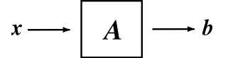
is mathematically analogous to an \(N\times N\) matrix \(A\) operating on a vector \(\boldsymbol{x} \in \mathbb{C}^{N}\) to produce another vector \(\boldsymbol{b} \in \mathbb{C}^{N}\) (see Matrices and LTI Systems for an overview).
\[\boldsymbol{A} \boldsymbol{x}=\boldsymbol{b} \nonumber \]

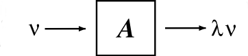
Just as an eigenvector (Section 14.2) of \(\boldsymbol{A}\) is a \(\boldsymbol{v} \in \mathbb{C}^{N}\) such that \(\boldsymbol{A v}=\boldsymbol{\lambda v}\), \(\boldsymbol{\lambda} \in \mathbb{C}\),

we can define an eigenfunction (or eigensignal) of an LTI system \(\mathcal{H}\) to be a signal \(f(t)\) such that
\[\mathcal{H}[f(t)]=\lambda f(t), \quad \lambda \in \mathrm{C} \nonumber \]

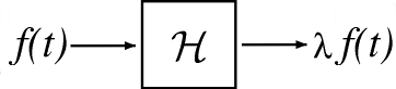
Eigenfunctions are the simplest possible signals for \(\mathcal{H}\) to operate on: to calculate the output, we simply multiply the input by a complex number \(\lambda\).
Eigenfunctions of any LTI System
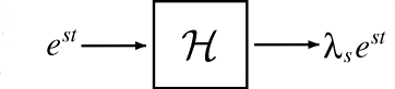
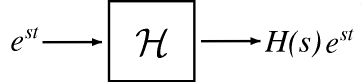
The class of LTI systems has a set of eigenfunctions in common: the complex exponentials (Section 1.8) \(e^{st}\), \(s \in \mathbb{C}\) are eigenfunctions for all LTI systems.
\[\mathcal{H}\left[e^{s t}\right]=\lambda_{s} e^{s t} \label{14.10} \]

Note
While \(\left\{e^{s t}, \quad s \in \mathbb{C}\right\}\) are always eigenfunctions of an LTI system, they are not necessarily the only eigenfunctions.
We can prove Equation \ref{14.10} by expressing the output as a convolution (Section 3.3) of the input \(e^{st}\) and the impulse response (Section 1.6) \(h(t)\) of \(\mathcal{H}\):
\[\begin{align}
\mathcal{H}\left[e^{s t}\right] &=\int_{-\infty}^{\infty} h(\tau) e^{s(t-\tau)} d \tau \nonumber \\
&=\int_{-\infty}^{\infty} h(\tau) e^{s t} e^{-(s \tau)} d \tau \nonumber \\
&=e^{s t} \int_{-\infty}^{\infty} h(\tau) e^{-(s \tau)} d \tau
\end{align} \nonumber \]
Since the expression on the right hand side does not depend on \(t\), it is a constant, \(\lambda_s\). Therefore
\[\mathcal{H}\left[e^{s t}\right]=\lambda_{s} e^{s t} \nonumber \]
The eigenvalue \(\lambda_s\) is a complex number that depends on the exponent \(s\) and, of course, the system \(\mathcal{H}\). To make these dependencies explicit, we will use the notation \(H(s) \equiv \lambda_{s}\).

Since the action of an LTI operator on its eigenfunctions \(e^{st}\) is easy to calculate and interpret, it is convenient to represent an arbitrary signal \(f(t)\) as a linear combination of complex exponentials. The Fourier series gives us this representation for periodic continuous time signals, while the (slightly more complicated) Fourier transform lets us expand arbitrary continuous time signals.