15.14: Approximation and Projections in Hilbert Space

Introduction

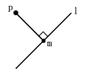
Given a line 'l' and a point 'p' in the plane, what's the closest point 'm' to 'p' on 'l'?

Figure \(\PageIndex{1}\): Figure of point 'p' and line 'l' mentioned above.

Same problem: Let \(x\) and \(v\) be vectors in \(\mathbb{R}^2\). Say \(\|v\|=1\). For what value of \(\alpha\) is \(\|x-\alpha v\|_{2}\) minimized? (what point in span{v} best approximates \(x\)?)

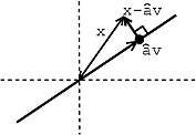
Figure \(\PageIndex{2}\)

The condition is that \(x-\widehat{\alpha} v\) and \(\alpha v\) are orthogonal.

Calculating α

How to calculate \(\widehat{a}\)?

We know that (\(x-\widehat{\alpha} v\)) is perpendicular to every vector in span{v}, so

\[\begin{array}{l}
\langle x-\widehat{\alpha} v, \beta v\rangle=0, \forall(\beta) \\
\bar{\beta}\langle(x, v)\rangle-\widehat{\alpha} \bar{\beta}\langle(v, v)\rangle=0
\end{array} \nonumber \]

because \(\langle v, v\rangle=1\), so

\[(\langle(x, v)\rangle-\hat{\alpha}=0) \Rightarrow(\hat{\alpha}=\langle x, v\rangle) \nonumber \]

Closest vector in span{v} = \(\langle(x, v)\rangle v\), where \(\langle(x, v)\rangle v\) is the projection of \(x\) onto \(v\).

We can do the same thing in higher dimensions.

Exercise \(\PageIndex{1}\)

Let \(V \subset H\) be a subspace of a Hilbert space (Section 15.4) \(H\). Let \(x \in H\) be given. Find the \(y \in V\) that best approximates \(x\). i.e., \(\|x-y\|\) is minimized.

Answer

1. Find an orthonormal basis \(\left\{b_{1}, \ldots, b_{k}\right\}\) for \(V\)
2. Project \(x\) onto \(V\) using \[y=\sum_{i=1}^{k}\left\langle\left(x, b_{i}\right)\right\rangle b_{i} \nonumber \] then \(y\) is the closest point in \(V\) to x and \((x-y) \perp V(\langle x-y, v\rangle=0, \quad \forall(v) \in V\)

Example \(\PageIndex{1}\)

\(x \in \mathbb{R}^{3}\), \(V=\operatorname{span}\left(\left\{\left(\begin{array}{l}
1 \\
0 \\
0
\end{array}\right),\left(\begin{array}{l}
0 \\
1 \\
0
\end{array}\right)\right\}\right)\), \(x=\left(\begin{array}{l}
a \\
b \\
c
\end{array}\right)\). So,

\[y=\sum_{i=1}^{2}\left\langle\left(x, b_{i}\right)\right\rangle b_{i}=a\left(\begin{array}{l}
1 \\
0 \\
0
\end{array}\right)+b\left(\begin{array}{l}
0 \\
1 \\
0
\end{array}\right)=\left(\begin{array}{l}
a \\
b \\
0
\end{array}\right) \nonumber \]

Example \(\PageIndex{2}\)

V = {space of periodic signals with frequency no greater than \(3w_0\)}. Given periodic f(t), what is the signal in V that best approximates f?

1. \(\left\{\frac{1}{\sqrt{T}} e^{j w_{0} k t}, k=-3,-2, \dots, 2,3\right\}\) is an ONB for V
2. \(g(t)=\frac{1}{T} \sum_{k=-3}^{3}\left\langle\left(f(t), e^{j w_{0} k t}\right)\right\rangle e^{j w_{0} k t}\) is the closest signal in V to f(t) ⇒ reconstruct f(t) using only 7 terms of its Fourier series.

Example \(\PageIndex{3}\)

Let V = {functions piecewise constant between the integers}

1. ONB for V.

\[b_{i}=\left\{\begin{array}{l}
1 \text { if } i-1 \leq t<i \\
0 \text { otherwise }
\end{array}\right. \nonumber \]

where \(\left\{b_{i}\right\}\) is an ONB.

Best piecewise constant approximation?

\[\begin{array}{c}
g(t)=\sum_{i=-\infty}^{\infty}\left\langle\left(f, b_{i}\right)\right\rangle b_{i} \\
\left\langle f, b_{i}\right\rangle=\int_{-\infty}^{\infty} f(t) b_{i}(t) \mathrm{d} t=\int_{i-1}^{i} f(t) \mathrm{d} t
\end{array} \nonumber \]

Example \(\PageIndex{4}\)

This demonstration explores approximation using a Fourier basis and a Haar Wavelet basis. See here for instructions on how to use the demo.