22.2: Investigation

Activity A: Business as usual scenario

Begin by launching C-ROADS in your web browser <https://www.climateinteractive.org/>. Figure 22.2.1 shows what you will first see when C-ROADS has finished launching.

Figure \(\PageIndex{1}\): The default screen for C-ROADS: Most of the controls for the simulator are in the upper left corner of the screen. Additional controls include the table in the lower right that controls the timing and rate of emission reductions, deforestation, and afforestation. The graph on the left shows \(CO_{2}\) emissions per year from 2000 to 2100 and the resulting increase in MGT (mean global temperature) for the same time period.

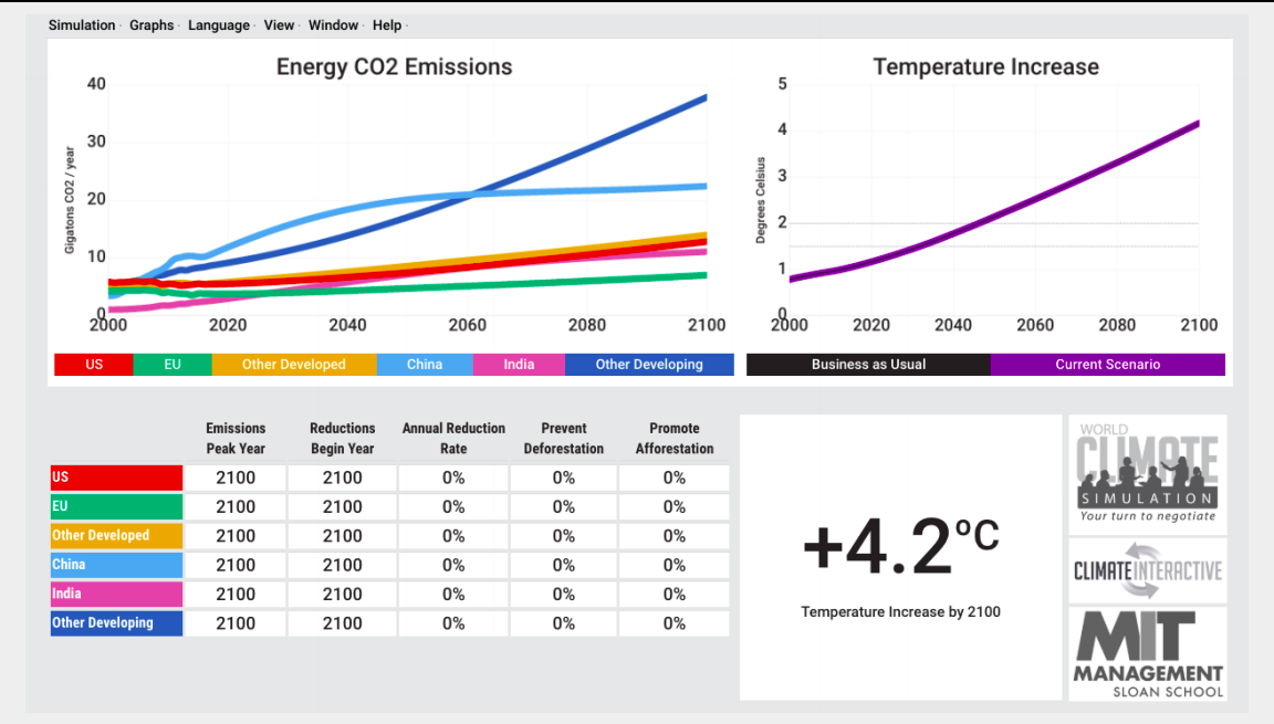
Note: C-ROADS does not work on browsers on mobile devices, so you will need to use either a laptop or a desktop computer to run it.

By default, C-ROADS begins with a “Business as usual” scenario or BAU. To understand what this means consider that approximately 85% of the energy consumed by global society comes from burning fossil fuels.

Also consider that global fossil fuel consumption has risen from 29,138 Twh in 1950 to 113,845 Twh in 2017. Under the BAU scenario, fossil fuels remain as the world’s dominant energy source with production and consumption continuing to increase at a similar or even faster rate than they did between 1950 and 2017. The goal of this activity is to become familiar with C-Roads and examine the climate impact of continuing with along the BAU pathway.

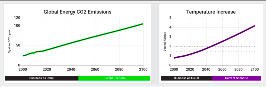
To begin, select “Global” from the drop down “Simulation” menu in the upper left corner of the screen. Once you do this you will see the graph on left change so it looks like Figure 22.2.2. The graph on the right should remain unchanged.

Figure \(\PageIndex{2}\): : Projected Global \(CO_{2}\) emissions from burning fossil fuels (left graph) and temperature increase above the pre-industrial average (right graph) from 2000 to 2100 under “Business as Usual” conditions. Move the cursor over the green or purple plot lines to read values for either emissions or temperature increase for specific years.

Questions - Business as Usual

1. What were the total emissions in the year 2000? What are they expected to be in 2020 and again in 2100?
2. What is the expected temperature increase in 2100?
3. What was the atmospheric \(CO_{2}\) concentration in 2000? What is it expected to be in 2020 and again in 2100?
   • To answer this go to the “Graphs” menu in the upper right and select “CO2 concentration” from the menu that appears when you scroll over “Impacts”.
4. What is the expected rise in sea level in 2020 and again in 2100?
   • This is sea level rise relative to 2000. To find this go the “Graphs” menu and select “Sea level rise” from the menu that appears when you scroll over “Impacts”.

Activity B: Paris commitments

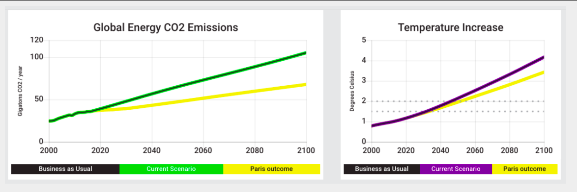
Another preset scenario in C-ROADS is the Paris Outcomes. These outcomes are based on the carbon reduction and sequestration commitments that signatories to 2015 Paris climate agreement brought to that international conference. To display this scenario, click on “Select Paris Outcomes” from the “View” menu in the upper right corner of the screen. What you see should look like Figure 22.2.3.

Figure \(\PageIndex{3}\): : Projected Global \(CO_{2}\) emissions and temperature increase for both the BAU and Paris Outcomes (yellow line) scenarios. You may have to go to the “Graphs” menu to select “Temperature Increase” from the “Impacts” sub menu to change the right graph to show temperature increase.

Questions - Paris 2015 Committments

1. For the Paris Outcomes what are the expected emissions in 2100?
2. For the Paris Outcomes, what are the expected atmospheric \(CO_{2}\) concentration, sea level, and ocean acidification in 2100?
3. How do all these values compare to the 2100 values from the BAU scenario?
4. How far above the temperature increase target set by the 2015 Paris climate agreement is the temperature increase resulting from the current reduction commitments?

The two dotted lines on the temperature increase graph represent the long-term commitment made in the 2015 agreement.

Activity C: Accelerated commitments

For this last activity you are going to experiment with what it would take to keep the 2100 MGT to between 1.5°C and 2.0°C above the pre-industrial MGT. You will be doing this by adjusting the timing and rate of emission reductions, deforestation, and afforestation.

• Emission reductions – Decreasing greenhouse gas emissions from energy production, manufacturing, agriculture, and other technological activities.
• Deforestation – Clearing forest for lumber and the creation of land for agriculture and other development. In short removing trees that would otherwise sequester carbon.
• Afforestation – Replanting cleared land in forest to provide a mean of carbon sequestration.

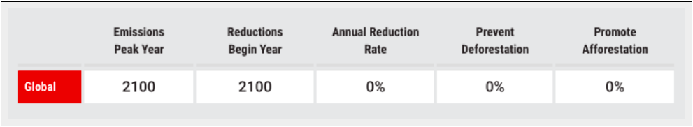
To begin make sure that your graphs look like Figure 22.2.3. This may require selecting “Global” and “Reset” from the “Simulation menu”, “Show Paris Outcomes” from the “View” menu, and “Temperature Increase” from the “Impacts” submenu of the “Graphs” menu.

Once your screen is set up, go to the table under the emissions graph (Figure 22.2.4) and click on the 2100 in the “Emissions Peak Year box. Change that value to 2060.

Figure \(\PageIndex{4}\): Controller for the timing and rate of emission reductions, deforestation, and afforestation.

Questions - Accelerated committment

1. What happens to the Global Energy \(CO_{2}\) Emissions (the green line) and 2100 temperature increase (purple line) when you set the Emissions Peak Year to 2060? Make sure to use numbers when you answer this.
2. What happens to the 2100 global emissions and temperature increase when you also set the Reductions Begin Year for 2060 and the Annual Reduction Rate to 5%?
3. What would it take to create each of the following scenarios?
4. The Temperature increase never goes above 2.0°C.
5. The temperature increase never goes above 1.5°C.
6. The temperature increase goes above 2.0°C but falls to 1.5°C by 2100.

For each scenario record the Emissions Peak Year, Reductions Begin Year, the Annual Reduction Rate, Prevent Deforestation, and Promote Afforestation necessary to achieve the goal. Make a table for this.