6.5: Locational Marginal Pricing

Locational Marginal Pricing

Unlike petroleum pipelines or natural gas pipelines, which in most cases require compression to maintain sufficient pressure to move product from the wellhead to the sales point, the cost of moving additional electrons through a network of conductors is essentially zero, since there is no fuel cost for “compression” in electrical networks.

(Actually, this isn’t quite true for a couple of reasons. First, transmission lines aren’t perfect conductors, so there is some resistance in the network. Because of this resistance, some of the electricity injected into the transmission grid by power generators is lost as heat between the power plant and the customer. The magnitude of these “resistive losses” is around 10% in a modern power grid like North America’s. What this means is that the system has to generate more power than is actually demanded, to account for these losses. For example, if demand in a system with 10% losses is 100 MW, then the system will need to generate around 111 MW. Second, the transmission grid needs to maintain a certain voltage level, and maintaining this level sometimes involves output adjustments at the power plant location, which does impose an economic cost on the system. In the discussion here, we will ignore these two costs to focus on the effects of transmission congestion.)

In the market-clearing example that we just went through, all suppliers were paid the market-clearing “system marginal price,” and the problem did not really say anything about where the generators or customers were located, or what the transmission network looked like. We just assumed that power produced at any one plant could be delivered to a customer at any location in the transmission network. Thus, electricity markets should exhibit the law of one price, just as we saw in natural gas networks.

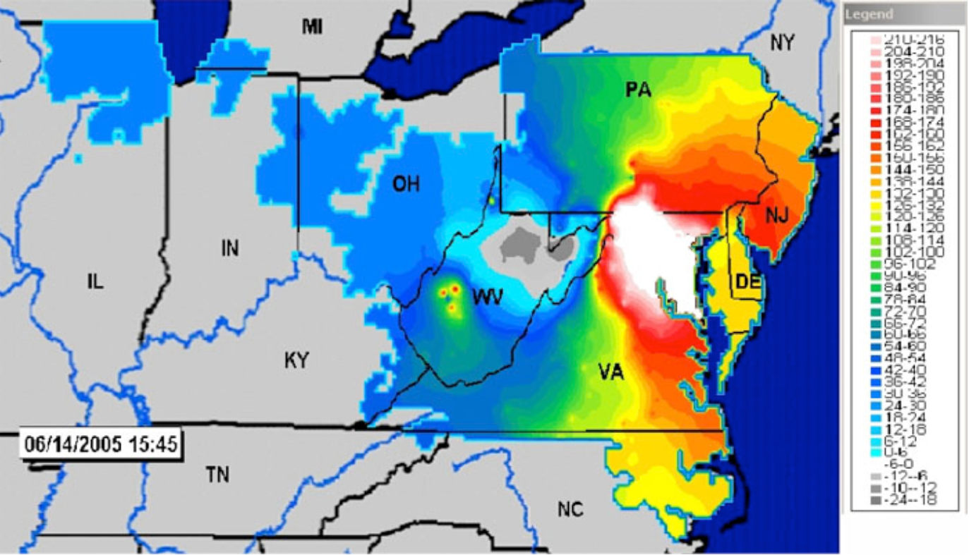
\(Figure \text { } 6.8\): Prices in the PJM electricity grid on June 14, 2005. Source: PJM.

While electricity markets should exhibit the law of one price, the reality is that they often do not. \(Figure 6.8\) shows a contour map of electricity prices in the PJM electricity grid on a warm, but not terribly hot day in June 2005. You can find more-up-to-date maps on the PJM website. You can also find a really nifty animation of LMPs from the MISO market. If you look carefully at the MISO animation, you may see some negative prices, meaning that someone using electricity gets paid to use it, and someone producing electricity actually pays to generate power! While this may seem strange, it is actually a natural economic outcome of a market with fluctuating supply and demand, and no storage. We'll get to the negative-price phenomenon later in the course.

Getting back to our picture of prices in the PJM system, you can see that prices in the western portion of PJM’s grid are an order of magnitude lower than prices in the eastern portion of the grid. This means that a power plant located in, say, Pittsburgh could make a lot of money by selling electricity to customers in Washington, DC. The demand from Washington should bid up the price in Pittsburgh as more generation in Pittsburgh comes online to serve the Washington market. This is just what we saw in our study of natural gas markets. But this doesn’t happen in electricity. Why?

The basic answer is “transmission congestion.” Conductors cannot hold an infinite number of electrons. At some point the resistive heat would just cause the conductor to melt. (Remember that materials expand when they get hot. When you hear about power lines “sagging” into trees, that is what’s going on.) So, power system engineers place limits on the amount of power that a transmission line can carry at any point in time. When a line’s loading hits its rated capacity, we say that the line is “congested” and it can’t transfer any additional power. So, the system has to find another way to meet demand, without additionally loading congested lines. Usually this involves reducing output at low-cost generators and increasing output at higher-cost generators. This process, known as “out of merit dispatch,” imposes an economic cost on the system.

After correcting for transmission congestion by adjusting the dispatch of power plants, the cost of meeting demand in one location (e.g., Washington) may be substantially higher than the cost of meeting demand in another location (e.g., Pittsburgh). The locational marginal price (LMP) at some particular point in the grid measures the marginal cost of delivering an additional unit of electric energy (i.e., a marginal MWh) to that location.

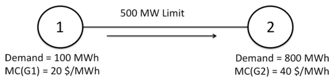
\(Figure \text { } 6.9\): Two-node network

We will illustrate the concept of LMP using the two-node network shown in \(Figure \text { } 6.9\). Node 1 has 100 MWh of demand, while node 2 has 800 MWh of demand. There are two generators in the system – one at node 1 with a marginal cost of $20/MWh and one at node 2 with a marginal cost of $40/MWh. A transmission line connects the two nodes. For the purposes of this example, assume that either of the generators could produce 1,000 MWh, and we will ignore any issues with transmission losses. Both generators submit supply offers to the electricity market that are equal to their marginal costs.

Suppose that the transmission line could carry an infinite amount of electricity. How should the system operator dispatch the generators to meet demand? Either generator by itself could meet all 900 MWh of demand in the system, so the system operator would dispatch generator 1 at 900 MWh and generator 2 would not be dispatched. The SMP would be equal to $20/MWh.

Now, suppose that the transmission line could carry only 500 MWh. In this case, the system operator could supply all of the demand at node 1 with generator 1, but only 500 MWh of demand at node 2 with generator 1. The remaining demand at node 2 would need to be met by dispatching generator 2. Since there is plenty of generation capacity left at generator 1, if demand at node 1 were to increase by 1 MWh, it could be met using generator 1 and thus the LMP at node 1 is $20 per MWh. If demand at node 2 were to increase, that demand would need to be met by increasing output at generator 2. Thus, the LMP at node 2 would be $40 per MWh.

Next we'll look at how much the Generators are paid and how much the Customers pay. Customers at Node 1 are charged $20 per MWh, while customers at Node 2 are charged $40 per MWh for all energy consumed. Generator 1 is paid $20 per MWh, while Generator 2 is paid $40 per MWh for all energy produced. You may notice here that while customers at Node 2 pay $40 per MWh for all 800 MWh that they consume, some of that energy was imported from Node 1 at a much lower cost. This is not a mistake - it's how the LMP pricing system works in the US.

The RTO collects revenue from the customers as follows:

From Node 1: 100 MWh × $20 per MWh = $2,000

From Node 2: 800 MWh × $40 per MWh = $32,000

Total Collections = $34,000

The RTO pays the generators as follows:

To Node 1: 600 MWh × $20 per MWh = $12,000

From Node 2: 300 MWh × $40 per MWh = $12,000

Total Collections = $24,000

The RTO collects excess revenue in the amount of $34,000 - $24,000 = $10,000. It collects this excess revenue because customers at Node 2 pay $40/MWh for all energy consumed, while some of those megawatt-hours only cost $20/MWh to produce.

This excess revenue is called "congestion revenue." In general, when there is congestion in the network and LMPs differ, then there will be some congestion revenue. We will discuss later in the course what the RTO does with this extra revenue. For now, just remember that whenever there is transmission congestion and LMPs at different nodes of the network aren't equal, the RTO will usually wind up with some congestion revenue.

As an exercise for yourself, calculate the LMPs and congestion revenue under a second two-node example. Demand at Node 1 is 5 MWh, while demand at Node 2 is 10 MWh. The transmission line connecting Nodes 1 and 2 has a capacity of 5 MWh. The marginal cost of Generator 1 is $10/MWh while the marginal cost of Generator 2 is $15/MWh.

You should find that the LMP at Node 1 is $10/MWh; the LMP at Node 2 is $15/MWh; and that 5 MW of power is exported from Node 1 to Node 2 on the transmission line.

You should also find that congestion revenue is equal to $25.