10.4: Decision Analysis Without Probabilities: Threshold and Sensitivity Analysis

Decision Analysis Without Probabilities: Threshold and Sensitivity Analysis

In the oil-field example from the previous section, the probabilities of a dry hole and a producer were known with confidence. This isn’t always true in the real world. Moreover, sometimes in real-world situations, there are so many possible outcomes that is impossible to assign a specific probability to each outcome. Suppose, just hypothetically, that oil prices could vary between $50 and $100 per barrel over the next five years. What is the probability that oil prices will average $50.03 per barrel? $50.04 per barrel? $99.30 per barrel?

In cases where determining probabilities explicitly is not possible or practical, threshold analysis and sensitivity analysis can be useful in understanding how the net present value of different alternatives may vary with some variation in key variables. Both of these techniques are useful in identifying situations under which one alternative is better than another. This can make even complex decision problems much more tractable for the decision-maker, since it reduces the problem from needing to calculate net present values for a large number of alternative outcomes to a judgment of whether one or another set of outcomes is more likely.

As we go through these techniques, we will often refer to something called a “parameter” in the decision problem. In this case, a parameter refers to a variable whose value affects the outcome of one or more alternatives – so a parameter is different from an alternative. In the oil field problem, the major parameter would be whether the field is a dry hole or whether it is a producer (so the parameter itself would be the probability of a producer versus a dry hole). The price of oil or the quantity of oil (if any) might be other important parameters for a problem such as this one.

Sensitivity analysis proceeds by selecting one parameter, changing its values, and observing how these new values change the net present value (or EMV) of some alternative. If sensitivity analysis is conducted using a small range of alternative values, or if the alternative values represent different scenarios, then it is sometimes (aptly) called “scenario analysis.”

We’ll illustrate this using the oil-field problem, performing a sensitivity analysis on the EMV of the drilling option as we vary the dry-hole probability. This analysis is pretty straightforward since we can write an expression for the EMV of drilling. We will need to use the fact that P(producer) = 1 – P(dry hole). (What rules of probability tell us that this is true?)

\(E M V(\text { Drill })=P(\text { dry hole }) \times-\$ 250,000+(1-P(\text { dry hole })) \times \$ 500,000\)

We can rearrange terms in the equation to get:

\(E M V(\text { Drill })=\$ 500,000-\$ 750,000 \times P(\text { dry hole })\)

This equation tells us a couple of things. First, the EMV of drilling is going to decline as the probability of a dry hole increases. This makes sense, since we lose money if we drill ourselves and the field is not a producer. Second, the relationship between EMV and the dry hole probability is linear, so the EMV falls at a constant rate as the dry hole probability increases. We can also use the equation to find the dry hole probability where the EMV is equal to zero. We do this by setting EMV(drill) equal to zero and manipulating the equation as follows:

\(\begin{array}{l}
0=\$ 500,000-\$ 750,000 \times P(\text { dry hole }) \\
P(\text { dry hole })=\$ 500,000 / \$ 750,000=\frac{2}{3}(67 \%)
\end{array}\)

Normally, sensitivity analysis is utilized to visualize the change in net present value or EMV with the change in some parameter of interest. For the drilling option, this is shown in \(Figure \text { } 10.2\), which plots the EMV versus the dry hole probability. Also shown in Figure 10.2 is the dry-hole probability where the EMV is equal to zero.

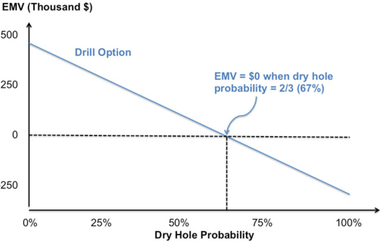
\(Figure \text { } 10.2\): A Dry Hole Probability Graph (EMV = 0)

As an exercise for yourself, perform the same sensitivity analysis on the option to farm-out. Your graph should look like the one in \(Figure \text { } 10.3\).

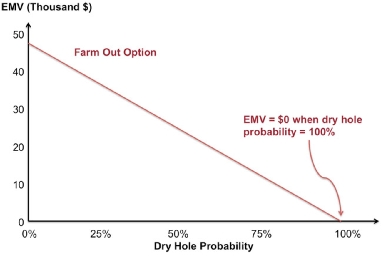
\(Figure \text { } 10.3\) - A Dry Hole Probability Graph (Farm Out Option)

Threshold analysis (also called break-point analysis) seeks to identify the value of a parameter where the best decision changes. Instead of asking what the probability of a producer versus a dry hole might be (and what are the associated EMVs of the option to drill or farm-out), a threshold analysis would ask how likely would it need to be for the field to be a producer for the expected-value decision-maker to choose the option to drill.

Threshold analyses can proceed graphically or algebraically. We will use the oil field example to illustrate both. Remember that the EMV of both the drilling and the farm-out options are functions of the dry-hole probability and of the NPVs for drilling and farming-out. Holding the NPVs constant as in \(Table \text { } 10.1\), we can write a mathematical expression for the EMV of each option as a function of the dry-hole probability P(dry hole). We will need to use the fact that P(producer) = 1 – P(dry hole). (What rules of probability tell us that this is true?)

\(\begin{array}{l}
E M V(\text { drill })=P(\text { dry hole }) \times-\$ 250,000+(1-P(\text { dry hole })) \times \$ 500,000 \\
E M V(\text { farm out })=P(\text { dry hole }) \times-\$ 0+(1-P(\text { dry hole })) \times \$ 50,000
\end{array}\)

If we graph the EMVs together on the same set of axes (as in \(Figures \text { } 10.2\) and \(10.3\)), the point at which the two lines cross would be the threshold. \(Figure \text { } 10.4\) illustrates this crossing point. Note that the scale of the axes, especially the horizontal axis, is different than in \(Figures \text { } 10.2\) or \(10.3\).

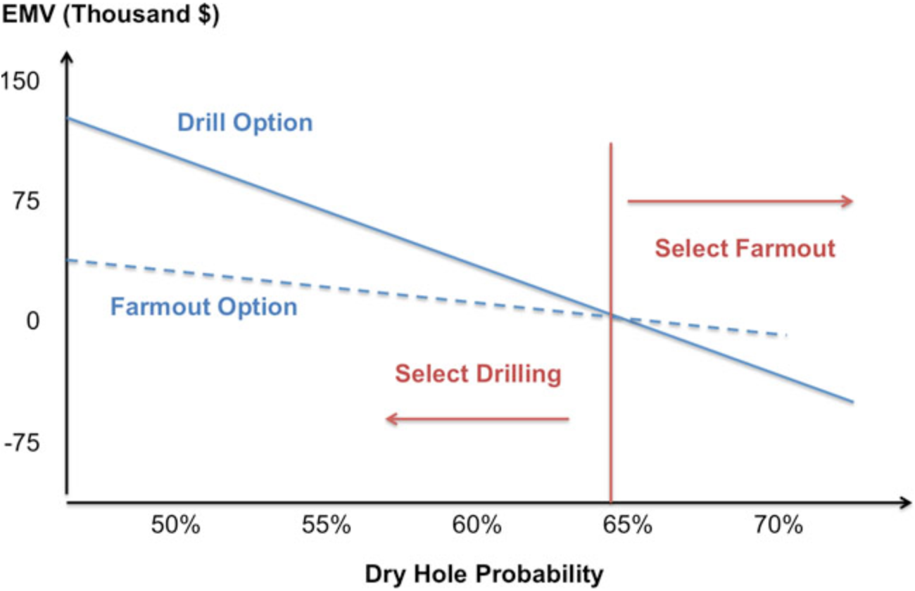
\(Figure \text { } 10.4\) - Dry Hole Probability (Crossing Point)

Looking carefully at \(Figure \text { } 10.4\), we can see that at a dry hole probability of around 65% or lower, the EMV of drilling is higher than the EMV of the farm-out option (this is why the drilling curve is above the farm-out curve). If the dry hole probability is above 65%, then the farm-out option has a higher EMV.

Algebraically, we can solve explicitly for the threshold value of the dry hole probability, by setting EMV(drill) equal to EMV(farm-out) and solving for the dry hole probability that makes these EMVs identical. Here we go!

\(\begin{array}{l}
E M V(\text { drill })=E M V(\text { farmout }) \\
\$ 500,000-\$ 750,000 \times P(\text { dry hole })=\$ 50,000-\$ 50,000 \times P(\text { dry hole }) \\
\$ 450,000=\$ 700,000 \times P(\text { dry hole }) \\
P(\text { dry hole })=0.64(64 \%)
\end{array}\)

Threshold analysis in particular can be a very powerful way of making difficult decisions seem more tractable. Even in the simple oil-field problem, the relevant question for the investor evaluating the oil-field decision is not to determine the exact probability of the field being a producer. The threshold analysis approach asks the potential investor whether they believe that there is more than a 65% chance of the field being dry. If so, then they should farm out drilling or not drill at all. If not, then the investor should choose to drill themselves.