
16: Gaseous Air Pollution
- Page ID
- 42040

\( \newcommand{\vecs}[1]{\overset { \scriptstyle \rightharpoonup} {\mathbf{#1}} } \)
\( \newcommand{\vecd}[1]{\overset{-\!-\!\rightharpoonup}{\vphantom{a}\smash {#1}}} \)
\( \newcommand{\id}{\mathrm{id}}\) \( \newcommand{\Span}{\mathrm{span}}\)
( \newcommand{\kernel}{\mathrm{null}\,}\) \( \newcommand{\range}{\mathrm{range}\,}\)
\( \newcommand{\RealPart}{\mathrm{Re}}\) \( \newcommand{\ImaginaryPart}{\mathrm{Im}}\)
\( \newcommand{\Argument}{\mathrm{Arg}}\) \( \newcommand{\norm}[1]{\| #1 \|}\)
\( \newcommand{\inner}[2]{\langle #1, #2 \rangle}\)
\( \newcommand{\Span}{\mathrm{span}}\)
\( \newcommand{\id}{\mathrm{id}}\)
\( \newcommand{\Span}{\mathrm{span}}\)
\( \newcommand{\kernel}{\mathrm{null}\,}\)
\( \newcommand{\range}{\mathrm{range}\,}\)
\( \newcommand{\RealPart}{\mathrm{Re}}\)
\( \newcommand{\ImaginaryPart}{\mathrm{Im}}\)
\( \newcommand{\Argument}{\mathrm{Arg}}\)
\( \newcommand{\norm}[1]{\| #1 \|}\)
\( \newcommand{\inner}[2]{\langle #1, #2 \rangle}\)
\( \newcommand{\Span}{\mathrm{span}}\) \( \newcommand{\AA}{\unicode[.8,0]{x212B}}\)
\( \newcommand{\vectorA}[1]{\vec{#1}} % arrow\)
\( \newcommand{\vectorAt}[1]{\vec{\text{#1}}} % arrow\)
\( \newcommand{\vectorB}[1]{\overset { \scriptstyle \rightharpoonup} {\mathbf{#1}} } \)
\( \newcommand{\vectorC}[1]{\textbf{#1}} \)
\( \newcommand{\vectorD}[1]{\overrightarrow{#1}} \)
\( \newcommand{\vectorDt}[1]{\overrightarrow{\text{#1}}} \)
\( \newcommand{\vectE}[1]{\overset{-\!-\!\rightharpoonup}{\vphantom{a}\smash{\mathbf {#1}}}} \)
\( \newcommand{\vecs}[1]{\overset { \scriptstyle \rightharpoonup} {\mathbf{#1}} } \)
\( \newcommand{\vecd}[1]{\overset{-\!-\!\rightharpoonup}{\vphantom{a}\smash {#1}}} \)
\(\newcommand{\avec}{\mathbf a}\) \(\newcommand{\bvec}{\mathbf b}\) \(\newcommand{\cvec}{\mathbf c}\) \(\newcommand{\dvec}{\mathbf d}\) \(\newcommand{\dtil}{\widetilde{\mathbf d}}\) \(\newcommand{\evec}{\mathbf e}\) \(\newcommand{\fvec}{\mathbf f}\) \(\newcommand{\nvec}{\mathbf n}\) \(\newcommand{\pvec}{\mathbf p}\) \(\newcommand{\qvec}{\mathbf q}\) \(\newcommand{\svec}{\mathbf s}\) \(\newcommand{\tvec}{\mathbf t}\) \(\newcommand{\uvec}{\mathbf u}\) \(\newcommand{\vvec}{\mathbf v}\) \(\newcommand{\wvec}{\mathbf w}\) \(\newcommand{\xvec}{\mathbf x}\) \(\newcommand{\yvec}{\mathbf y}\) \(\newcommand{\zvec}{\mathbf z}\) \(\newcommand{\rvec}{\mathbf r}\) \(\newcommand{\mvec}{\mathbf m}\) \(\newcommand{\zerovec}{\mathbf 0}\) \(\newcommand{\onevec}{\mathbf 1}\) \(\newcommand{\real}{\mathbb R}\) \(\newcommand{\twovec}[2]{\left[\begin{array}{r}#1 \\ #2 \end{array}\right]}\) \(\newcommand{\ctwovec}[2]{\left[\begin{array}{c}#1 \\ #2 \end{array}\right]}\) \(\newcommand{\threevec}[3]{\left[\begin{array}{r}#1 \\ #2 \\ #3 \end{array}\right]}\) \(\newcommand{\cthreevec}[3]{\left[\begin{array}{c}#1 \\ #2 \\ #3 \end{array}\right]}\) \(\newcommand{\fourvec}[4]{\left[\begin{array}{r}#1 \\ #2 \\ #3 \\ #4 \end{array}\right]}\) \(\newcommand{\cfourvec}[4]{\left[\begin{array}{c}#1 \\ #2 \\ #3 \\ #4 \end{array}\right]}\) \(\newcommand{\fivevec}[5]{\left[\begin{array}{r}#1 \\ #2 \\ #3 \\ #4 \\ #5 \\ \end{array}\right]}\) \(\newcommand{\cfivevec}[5]{\left[\begin{array}{c}#1 \\ #2 \\ #3 \\ #4 \\ #5 \\ \end{array}\right]}\) \(\newcommand{\mattwo}[4]{\left[\begin{array}{rr}#1 \amp #2 \\ #3 \amp #4 \\ \end{array}\right]}\) \(\newcommand{\laspan}[1]{\text{Span}\{#1\}}\) \(\newcommand{\bcal}{\cal B}\) \(\newcommand{\ccal}{\cal C}\) \(\newcommand{\scal}{\cal S}\) \(\newcommand{\wcal}{\cal W}\) \(\newcommand{\ecal}{\cal E}\) \(\newcommand{\coords}[2]{\left\{#1\right\}_{#2}}\) \(\newcommand{\gray}[1]{\color{gray}{#1}}\) \(\newcommand{\lgray}[1]{\color{lightgray}{#1}}\) \(\newcommand{\rank}{\operatorname{rank}}\) \(\newcommand{\row}{\text{Row}}\) \(\newcommand{\col}{\text{Col}}\) \(\renewcommand{\row}{\text{Row}}\) \(\newcommand{\nul}{\text{Nul}}\) \(\newcommand{\var}{\text{Var}}\) \(\newcommand{\corr}{\text{corr}}\) \(\newcommand{\len}[1]{\left|#1\right|}\) \(\newcommand{\bbar}{\overline{\bvec}}\) \(\newcommand{\bhat}{\widehat{\bvec}}\) \(\newcommand{\bperp}{\bvec^\perp}\) \(\newcommand{\xhat}{\widehat{\xvec}}\) \(\newcommand{\vhat}{\widehat{\vvec}}\) \(\newcommand{\uhat}{\widehat{\uvec}}\) \(\newcommand{\what}{\widehat{\wvec}}\) \(\newcommand{\Sighat}{\widehat{\Sigma}}\) \(\newcommand{\lt}{<}\) \(\newcommand{\gt}{>}\) \(\newcommand{\amp}{&}\) \(\definecolor{fillinmathshade}{gray}{0.9}\)Learning Objectives
After completing this chapter, you will be able to
- Outline the major sources of emission of air pollutants associated with sulphur, nitrogen, and hydrocarbons.
- Explain the difference between primary and secondary pollutants.
- Contrast the environmental problems associated with stratospheric and tropospheric ozone.
- Examine the importance of air pollutants to ecosystems and to human health.
- Outline the lessons to be learned from natural pollution at the Smoking Hills.
- Describe the patterns of pollution and ecological damage near point sources of air pollution.
Introduction
Gaseous air pollutants are emitted from various natural sources, such as volcanoes and forest fires. However, anthropogenic emissions of some gases may be greater than the natural ones, and are increasing because of population growth and industrialization.
In ancient times, there was not much pollution. Nevertheless, even then local problems would have occurred. For instance, smoky wood fires used for cooking and warmth would likely have caused poor-quality air to occur inside of badly ventilated dwellings. Hunting cultures often used fire to drive game animals and improve local forage, and those burns would have resulted in large emissions of particulate carbon (soot), carbon dioxide, and other gases that would have temporarily impaired air quality. Overall, however, these effects were relatively minor.
Of course, as people became more numerous and industrialized, air pollution increasingly developed into a much bigger problem. When the Industrial Revolution began (around 1750), coal quickly became the major fuel used to generate heat and energy for machines, and that resulted in increasingly worse air pollution. The widespread use of coal led to severe pollution by sulphur dioxide (SO2) and soot in the industrial towns and cities of Europe and the Americas. Since 1900, burgeoning industrialization and new technologies such as power plants and automobiles have further increased the emissions of pollutants.
Air pollution can be especially severe in situations when the lower atmosphere is stable and calm. These conditions often occur beneath an atmospheric phenomenon called an inversion, in which a layer of cool air is trapped beneath a higher layer of warmer air (the more usual pattern is for temperature to cool with increasing altitude). An atmospheric inversion is a relatively stable condition that prevents polluted ground-level air from mixing with cleaner air from higher altitudes (see In Detail 16.1). If an atmospheric inversion is accompanied by fog, the pollution is known as smog (a word derived from “smoke” and “fog”). As recently as the 1950s, occasional so-called “killer smogs” rich in SO2 and soot caused the deaths of thousands of urban people, and many more suffered from respiratory distress (pollution rich in SO2 is also called reducing smog). The most famous killer smogs occurred in London, Glasgow, some other industrial centres of Europe, and near Pittsburgh in the United States (these are described later).
Once scientists recognized the severe damage that was being caused by air pollution, governments began to pass laws to decrease the emissions. Pollution control became particularly vigorous after medical researchers discovered clear evidence of links between air quality and human diseases and deaths. Particular attention was paid to air pollution in urban environments, where the killer smogs were most frequent. Governments typically responded with important control actions, such as the following:
- switching from coal, which is a relatively “dirty” fossil fuel, to “cleaner” ones such as natural gas or oil, or to alternative energy technologies such as nuclear power and hydroelectricity
- constructing tall smokestacks to spread emissions over a much wider area so that ground-level exposures become less common and less intense – this tactic is the “dilution solution to pollution”
- centralizing energy production in large power plants to replace much of the relatively dirty and inefficient burning of coal in home fireplaces and furnaces, thereby permitting better control of emissions
- treating waste gases to remove some of their pollutant content, thereby reducing emissions to the atmosphere
Because of these helpful regulatory actions, the importance of reducing smogs became much less in many countries. However, so-called oxidizing smog has become more important causes of damage in many regions. Oxidizing smog develops in the atmosphere through complex photochemical reactions in which hydrocarbons and nitrogen oxides are transformed into ozone (O3) and other gases. Ozone and other oxidizing gases harm vegetation and irritate the respiratory system and eyes of people. Oxidizing smog develops under sunny conditions if hydrocarbons and nitrogen oxides are present from automobile and industrial emissions, and especially if the presence of an atmospheric inversion reduces dispersion of the polluted air mass.
In this chapter, we examine the most important gaseous pollutants. Their sources of emission, chemical transformations, and toxicity are described, and Canadian case studies are used to demonstrate the ecological damages that may be caused.
In Detail 16.1. Normally, the temperature of the atmosphere decreases with increasing altitude. Under certain conditions, however, a layer of relatively cool air may become trapped under a layer of warmer air, a phenomenon known as an atmospheric inversion (or temperature inversion; see Figure).
Figure 16.1. Normally, air temperature decreases with increasing altitude (red line), but during an atmospheric inversion, a ground-level layer of cooler air is trapped beneath warmer air (blue lines).
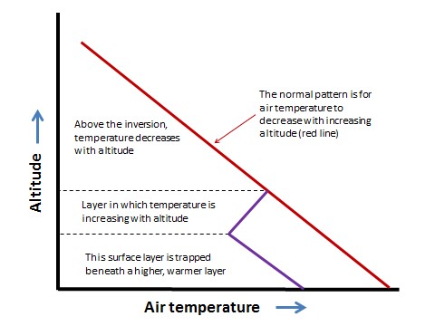
An atmospheric inversion may develop on a clear, cloudless night. Under such conditions, the ground surface cools quickly as it radiates heat that was absorbed during the day. This can result in a layer of cool air occurring beneath a higher layer of warmer air. Hilly terrain is particularly vulnerable to developing atmospheric inversions because relatively dense cool air can flow downward from hilltops and accumulate in valleys. Sometimes during the summer, stable atmospheric conditions may develop at higher altitude, capping a still-mixing air mass at ground level.
An atmospheric inversion can be rather stable. Until it is dispersed by vigorous winds, it can trap and accumulate air pollutants that are emitted during the inversion event. Severe episodes of air pollution can occur when stable inversions develop and are maintained for several days.
Some places regularly develop less-persistent inversions, such as Los Angeles, Mexico City, and Greater Vancouver. In these places, the inversions develop in the morning but are typically dispersed during the afternoon. In the meantime, however, oxidizing air pollutants such as ozone can accumulate into a photochemical smog.
Sulphur Gases
Emissions and Transformations
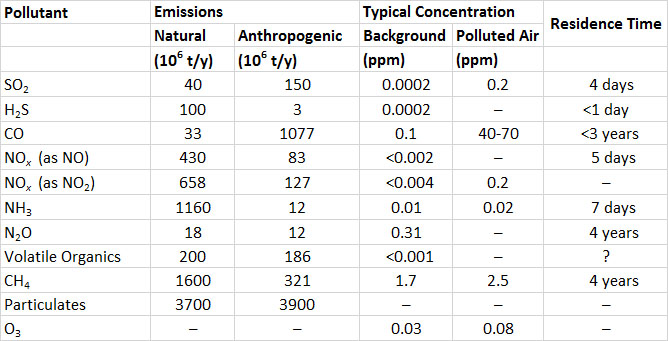
Sulphur dioxide (SO2) is one of the most important of the gaseous air pollutants. SO2 is a colourless but pungent gas. Humans can detect its bitter taste at a concentration of only 0.3-1 ppm (parts per million; for SO2, 1 ppm = 2.6 mg/m3). Hydrogen sulphide (H2S), another sulphur gas, can be detected as a foul odour, reminiscent of rotten eggs, at concentrations lower than 1 ppb (parts per billion; for H2S, 1 ppm = 1.4 mg/m3) (unless otherwise indicated, specific data cited in this and other chapters in this section on environmental damages are from Freedman, 1995).
After they are emitted to the atmosphere, SO2 and H2S become oxidized to other compounds, and ultimately form sulphate (SO42–; see In Detail 16.2). Because the sulphate ion carries negative charges, it is an anion (this refers to any ion, atom, or molecule with a negative charge). Because H2S is quickly oxidized to SO2, its atmospheric residence time is less than one day (this is the time to complete disappearance of an initial amount). SO2 oxidizes more slowly, at a rate of < 1-5% per hour, depending on sunlight, humidity, strong oxidants such as ozone, and the presence of metal-containing particulates that may act as catalysts. A typical residence time of SO2 in the atmosphere is about four days. Consequently, SO2 may disperse a long distance from its point of emission before it becomes oxidized or is deposited to a terrestrial or aquatic surface. This kind of dispersal is referred to as long-range transportation of air pollution (LRTAP).
Atmospheric sulphate, formed by the oxidation of SO2 or H2S, can combine with positively charged ions (cations) to form various compounds. Most atmospheric sulphate occurs as tiny particulates, especially ammonium sulphate ((NH4)2 SO4). This is the most prominent component, along with ammonium nitrate (NH4NO3), of the fine particulate haze that often impairs visibility in cities. Haze also occurs in some rural areas where pollutants have been imported by LRTAP from emission sources elsewhere. Other cations that combine with sulphate include calcium (Ca2+), magnesium (Mg2+), and sodium (Na+). Often, however, there are not enough of these cations to balance all of the negative charges of the sulphate (SO42–) present. Under such conditions, hydrogen ions (H+) serve to balance some of the negative charges, resulting in an aerosol containing sulphuric acid (H2SO4), the most important component of acidic precipitation (see Chapter 19).
Emissions of Sulphur Gases
Volcanoes are natural sources of emission of sulphur gases. On average, volcanoes emit about 12-million tonnes of sulphur gases per year, of which 90% is SO2 and 10% is H2S. However, the enormous 1991 eruption of Mount Pinatubo in the Philippines emitted 7-10-million tonnes of SO2 (expressed as the sulphur content, or SO2-S). The much smaller eruption of Mount St. Helens in Washington State in 1980 vented about 0.2-million tonnes of SO2-S. Natural emissions of SO2 also occur during wildfires.
The global anthropogenic emissions of SO2 are about 150-million tonnes per year, or 3.8-times the natural releases (Table 16.1). Fossil-fuel combustion accounts for about half of the anthropogenic emissions. Coal and petroleum contain mineral compounds of sulphur, such as pyrite (FeS2), as well as organic sulphur compounds. When these fuels are burned, the sulphur becomes oxidized to gaseous SO2, which may be vented to the atmosphere. Hard coals mined in eastern North America contain 1-12% sulphur, softer coals from western regions have <0.3-1.5%, crude oil has 0.8-1.0% residual fuel oils such as bunker -C have 0.3-0.4%, and motor fuels such as diesel and gasoline have 0.04-0.05%. Other important sources of SO2 emissions are manufacturing processes (23% of global emissions), the smelting of metal ores (7%), and the burning of natural habitats during agricultural conversions (most of the rest).

Anthropogenic emissions of SO2 have increased enormously since the beginning of the Industrial Revolution. Emissions in 1860 were about 5-million tonnes, compared with about 150-million tonnes in 2000. Since then, most of the wealthier countries have invested heavily in clean-air technologies for power plants and other industrial users of coal and oil in order to reduce emissions of damaging SO2 to the atmosphere. The clean-air actions include the following:
- the installation of technologies to capture SO2 from post-combustion waste gases (this is known as flue-gas desulphurization or scrubbing)
- the removal of some of the sulphur content of fuels (known as fuel desulphurization or coal washing)
- the installation of particulate-control devices (such as electrostatic precipitators) to greatly reduce the emissions of particulates (although this has little effect on SO2 emissions)
- switching to low- or no-sulphur fuels such as natural gas, or to no-sulphur energy technologies such as hydroelectricity and nuclear power (known as fuel-switching)
- energy conservation to reduce the overall demand for fuel and associated emissions of pollutants
- building taller smokestacks to disperse emissions of SO2 more widely, which helps to decrease the local ground-level pollution
However, future global emissions are bound to increase. China, India, and other rapidly industrializing countries supply much of their burgeoning energy needs by burning coal and petroleum fuels. In China, coal is the major source of industrial energy, accounting for 68% of the energy supply (in 2013; Table 13.9). Due to increasing industrialization, emissions of SO2 in China increased from 10-million tonnes in 1980 to 34-million tonnes in 2000, a 3.4-fold increase in only 20 years.
The amounts of SO2 emissions differ greatly among nations, depending on their population, their kind of industrialization, and the fuels they mostly use. For instance, Canadian emissions of SO2 are about 22% of those of the United States (Table 16.2). However, the population of Canada is only about 11% that of the United States (Chapter 10). Therefore, per-capita emissions of SO2 are about double in Canada than in the United States.
About 66% of Canadian emissions of SO2 are from large industrial sources, particularly metal smelters, while 24% are from “fuel combustion,” which is mostly fossil-fuelled power plants. In comparison, 84% of U.S. emissions are from power plants, and 10% from industrial sources. Most of this difference is due to two factors: a relatively large proportion of electricity generation in Canada is from nuclear and hydro technologies, which do not emit SO2, and metal smelting is a major industry in Canada.
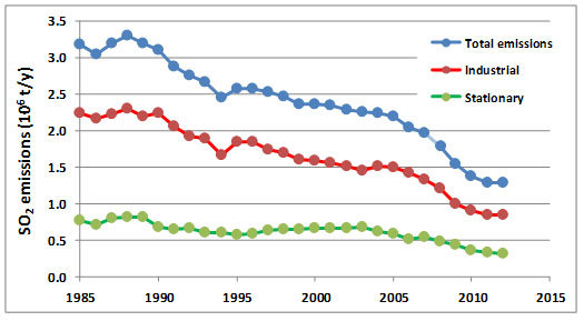
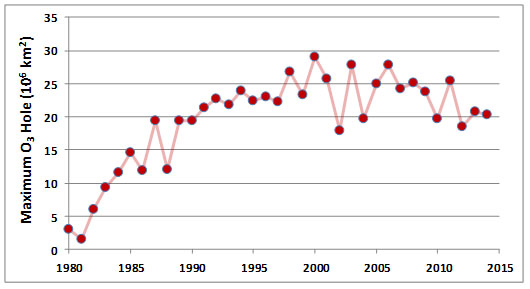
Because of human-health and environmental damages associated with SO2 and other air pollutants, most developed nations have acted to reduce their emissions. In Canada, emissions of SO2 were reduced by about 41% between 1985 and 2012 (Figure 16.1), compared with a 32% reduction in the United States. In both countries the reductions were achieved by several methods:
- switching to low- or no-sulphur fuels for some major uses, especially for electricity generation
- removing sulphur from some fuels prior to combustion, mostly by coal washing
- reducing energy demands through conservation
- installing scrubbers to remove SO2 from post-combustion waste gases before they are vented to the atmosphere
However, as is shown in Figure 16.1, reductions of emissions from industrial sources (especially metal smelters) and stationary sources (mostly coal-fuelled power plants) have been especially important. The large reductions of SO2that have been achieved in North America during the past several decades cost many billions of dollars to achieve, and they should be regarded as an important “success story” of pollution control.
In contrast to SO2, the global emissions of sulphide gases are mostly from natural sources (Table 16.1). The largest sources are H2S emitted from anoxic sediment in shallow marine and inland waters, and dimethyl sulphide ((CH3)2S) produced by phytoplankton and out-gassed from oceanic waters. The natural emission of H2S is about 100-million tonnes per year, and dimethyl sulphide, 15-million tonnes per year (both expressed as sulphur equivalent, or as tonnes of S). Anthropogenic emissions of H2S are about 3-million tonnes per year, and are mostly from chemical industries, sewage-treatment plants, and livestock manure.
The global emission of all sulphur-containing gases is equivalent to almost 300- million tonnes of sulphur per year. About half of the global emission is from anthropogenic sources.
Clean air typically contains less than 0.2 ppb of SO2 or H2S. Concentrations of SO2 and H2S in air that is polluted by emissions are highly variable. They are typically about 0.2 ppm in urban atmospheres but can exceed 3 ppm close to large emission sources.
Toxicity of Sulphur Gases
Concentrations of H2S in the environment are rarely high enough to be toxic to plants. However, accidental emissions from sour-gas plants (where H2S is removed from natural gas) may cause local vegetation damage. In contrast, concentrations of SO2 in cities and near industrial sources are often high enough to injure wild and cultivated plants. Near certain metal smelters, vegetation has been severely damaged, as we examine later.
An exposure to 0.7 ppm SO2 for one hour will result in acute injury to most plant species, as will 0.2 ppm over an eight-hour period. It is important to note, however, that certain species are extremely sensitive to SO2 exposures (they are hypersensitive) and can suffer acute injuries at concentrations lower than those just noted.
In addition, plants will often exhibit a reduction in yield when exposed to concentrations of SO2 that are lower than those required to cause an acute injury. This type of response, which occurs without symptoms of acute tissue damage, is referred to as “hidden injury”. Hidden injuries to wild and agricultural vegetation are measured by enclosing plants in experimental chambers and exposing them to either air containing ambient levels of SO2, or that that has been filtered through charcoal to remove that gas. If productivity is greater in the filtered air, it follows that the ambient SO2 was causing a hidden injury. Studies of pasture grasses have found that exposure to SO2 concentrations averaging only 0.04 ppm would cause hidden injuries as reductions of yield.
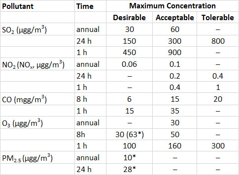
The Canadian air-quality guideline for ambient SO2 in the atmosphere is a maximum of 450 µg/m3 (0.17 ppm) over a one-hour exposure (Table 16.3). This guideline is based on the concentration that causes acute foliar (leaf) injuries to most agricultural plants. Although regions meeting this guideline would not show much acute damage to vegetation, relatively sensitive species might be affected through hidden injuries, possibly resulting in significant losses of yield.
Humans and most other animals are much less sensitive to SO2 than plants are. Guidelines for allowable exposures of people to SO2 and other potentially toxic gases accommodate the fact that, in terms of dose received, longer-term exposures to low concentrations can be as important as higher acute exposures.
Guidelines for occupational exposures to air pollutants are frequently greater than those for ambient exposures. In North America, it is recommended that occupational exposures to SO2 be no higher than 2 ppm (5.2 mg/m3) over the long term, and no higher than 5 ppm (13 mg/m3) for shorter exposures. However, some people are relatively sensitive to SO2, and concentrations less than 1 ppm (2.6 mg/m3) may cause them to suffer asthma or other distresses related to impaired lung function. In addition, some studies have suggested that long-term exposures of large human populations to sulphate particulate aerosols (which are ultimately derived from gaseous SO2) in cities may result in small increases in the incidence of respiratory and circulatory diseases, most probably in hypersensitive people.
In Detail 16.2. Air Pollution Chemistry
Air pollutants are emitted as particular chemicals, which may then be transformed into other compounds through reactions occurring in the atmosphere. Several examples follow.
Oxidation of SO2
SO2 + OH → HO•SO2 (1)
HO•SO2 + O2 → HO2 + SO3 (2)
SO3 + H2O → H2SO4 (3)
H2SO4 → 2H+ + SO42- (in aqueous solution) (4)
Note that the SO42– produced is important as a constituent of acid rain and as particulate ammonium sulphate ((NH4)2SO4), which are important pollutants.
Oxidation of NO
NO + HO2 → NO2 + OH (5)
NO2 + OH → HNO3 (6)
HNO3 → H+ + NO3– (in aqueous solution) (7)
Similarly, the NO3– produced is important in acid rain and as particulate ammonium nitrate (NH4NO3).
Formation and Destruction of Stratospheric O3
O2 + UV radiation → O + O (8) O + O → O2 (9)
O + O2 → O3 (10)
O3 + UV radiation → O2 + O (11)
Reaction 11 is an ultraviolet photodissociation of O3. Ozone can also be consumed by reactions with NO, NO2, N2O, and with ions or simple molecules of chlorine (especially ClO), bromine, and fluorine. These reactions are too complex to describe here.
Formation and Destruction of Ground-Level O3
O + O2 → O3 (10)
NO2 + UV radiation → NO + O (12)
NO + O3 → NO2 + O2 (13)
NO + RO2 → NO2 + RO (14)
The formation of O3 (reaction 10) requires atomic O, formed by the photodissociation of NO2 (reaction 12). Ozone can be consumed by reaction with NO (an emitted gas), which regenerates NO2 (reaction 13). Atmospheric O3 can, however, accumulate if other reactions (such as reaction 14) convert NO to NO2, because these operate in competition with reaction 13 for NO. (The species RO2 includes various chemicals known as peroxy radicals, formed by the degradation of organic molecules by reaction with hydroxyl radicals, followed by the addition of molecular O2. RO is the chemically reduced form of RO2.)
Nitrogen Gases
Emissions and Transformations
The most important of the nitrogen-containing gases are nitric oxide (NO), nitrogen dioxide (NO2), nitrous oxide (N2O), and ammonia (NH3). NO and NO2 are often considered together as a complex, referred to as NOx.
Ammonia (NH3), a colourless gas, is emitted mostly from wetlands, where it is produced during the anaerobic decomposition of dead biomass. Natural emissions of NH3 are about 1.2-billion tonnes per year (Table 16.1). Sources of anthropogenic emissions include fossil-fuel combustion (4-million tonnes per year) and animal husbandry (0.2-million tonnes per year). The residence time of NH3 in the atmosphere is about seven days (the NH3 is eventually oxidized to nitrate).
Nitrous oxide (N2O) is a colourless, non-toxic gas that produces a mild euphoria when inhaled. This gas is also known as “laughing gas” and is used as a mild anaesthetic in medicine, and sometimes as a recreational drug. Because N2O is a rather unreactive compound, it has a long residence time in the atmosphere of about four years. Most N2O emissions are associated with microbial denitrification in soil and water. These are equivalent to about 18-million tonnes per year, while industrial emissions are 12-million tonnes per year. Agricultural soil fertilized with nitrate can have high rates of N2O emission, and modern agricultural practices are thought to have increased global emissions by about 40%.
Nitric oxide (NO) is a colourless and odourless gas, while nitrogen dioxide is reddish, pungent, and irritating to respiratory and eye membranes. Natural emissions of NOx are about 430-million tonnes per year (expressed as NO; the same emissions expressed as NO2 are 658-million tonnes per year). The most important natural emissions of NOx are due to bacterial denitrification of nitrate in soil, fixation of atmospheric nitrogen gas (N2) by lightning, and oxidation of biomass nitrogen during fires (see Chapter 5).
Anthropogenic emissions of NOx, about 83-million tonnes per year (expressed as NO), result mostly from the combustion of fossil fuels, especially in automobiles and power plants (Table 16.1). These emissions are mostly NO, which is secondarily oxidized to NO2 by reactions in the atmosphere. Ultimately, most atmospheric NOx gases become oxidized to nitrate (NO3–), an ion that is important in the acidification of precipitation and ecosystems (Chapter 19).
Toxicity of Nitrogen Gases
It is rare that concentrations of NH3 or NOx gases are high enough to injure vegetation. The environmental damage associated with NOx is focussed on the photochemical reactions by which ozone, a much more toxic gas, is produced (see below), and also the acidification of precipitation and ecosystems.
Ambient concentrations of NH3 and NOx are rarely high enough to bother humans. Guidelines for long-term exposures in an occupational setting are 25 ppm (34 mg/m3) for NO and 5 ppm (10 mg/m3) for NO2. Occupational guidelines for short-term exposures are 35 ppm (47 mg/m3) and 5 ppm (10 mg/m3), respectively. Intense occupational exposures to NOx can cause impaired pulmonary function in humans.
Organic Gases and Vapours
Emissions and Transformations
Hydrocarbons are a diverse group of chemicals whose molecular structures containing various combinations of hydrogen and carbon atoms. The simplest hydrocarbon is methane (CH4), a gas. Larger hydrocarbons with greater weight and more complex structure may occur as vapors, liquids, or solids (Chapter 22). Other volatile organic compounds (VOCs) may contain oxygen, nitrogen, and other light elements in addition to carbon and hydrogen, and include alcohols, aldehydes, and phenols.
The background concentration of methane in the atmosphere is about 1.7 ppm (1 ppm = 0.65 mg/m3), while all other hydrocarbons and volatile organics together amount to less than 1 ppb (Table 16.1; the conversions to mg/m3 are variable depending on the molecular weight). Most emissions of CH4 are natural and are associated with the fermentation of organic matter by microbes in anaerobic wetlands. Smaller amounts are out-gassed from deposits of fossil fuels, during wildfires, and from burping and flatulent ruminant animals (such as cows and sheep) and termites, which produce CH4 as they digest their plant foods. The global natural emissions of CH4 are about 1.6-billion tonnes per year, and the natural emissions 0.3-billion tonnes per year.
Atmospheric hydrocarbons other than CH4 are referred to as non-methane hydrocarbons. Natural emissions of these and many organics occur mainly as gases and vapors that evaporate from living vegetation, along with smaller quantities that out-gas from deposits of fossil fuels. The largest emissions from forests typically occur during hot, sunny days. Natural emissions of non-methane hydrocarbons are about 200-million tonnes per year, compared with anthropogenic emissions of 186-million tonnes per year (Table 16.1). The most important anthropogenic sources are unburned fuel emitted from vehicles and aircraft, releases during fossil-fuel mining and refining, and evaporation of solvents.
Toxicity of Organic Gases and Vapours
Organic gases and vapors can be toxic, but atmospheric concentrations are rarely high enough to damage vegetation or animals. The environmental importance of these gases and vapors lies mainly in their role in the photochemical reactions that produce toxic ozone. In addition, CH4 is an important greenhouse gas that affects global warming (Chapter 17). In some workplaces, however, relatively toxic organics such as benzene and formaldehyde may be important pollutants.
Ozone
There are two different ozone-related environmental issues: (1) O3 in the stratosphere and (2) O3 in the troposphere (ground-level ozone). High concentrations of ozone are naturally present in the upper-atmospheric layer known as the stratosphere, which begins at about 8-17 km above the Earth’s surface, depending on the latitude and season. Stratospheric O3 causes no damage and is not an air pollutant. Rather, by absorbing solar ultraviolet radiation, stratospheric 3helps to protect organisms on the surface pf the planet from many damaging effects of exposure to this harmful part of the electromagnetic spectrum. In contrast, O3 in the lower3 atmosphere (the troposphere) is an important air pollutant that is damages vegetation, materials, and human health. Ozone is removed from the atmosphere by interactions with other gases, organic vapors, and terrestrial and aquatic surfaces (including vegetation).
Ground-Level Ozone
Ground-level ozone (O3) is the most damaging of the so-called photochemical air pollutants. Less important are peroxyacetyl nitrate (PAN), hydrogen peroxide (H2O2), and other oxidant gases. Oxidizing smog is rich in O3 and the other oxidant gases. These chemicals are secondary pollutants, meaning they are not actually emitted to the atmosphere (as are primary pollutants such as SO2 and NOx). Instead, they are synthesized within the atmosphere by photochemical reactions (chemical reactions that require light, especially ultraviolet wavelengths). These proceed at faster rates and result in a buildup of oxidants if NOx and hydrocarbons are present in high concentrations, a condition that is typically due to anthropogenic emissions.
Some regions tend to develop a weak atmospheric inversion in the morning. Because an inversion is relatively stable and resists the in-mixing of cleaner air from above or beyond, this condition encourages the development of oxidizing smog during the morning and early afternoon. Later in the day, the inversion is typically broken up by stronger winds, and the air pollution is dispersed. Such inversions and their ozone-rich smog are common phenomena around the Los Angeles basin, Mexico City, Vancouver, and elsewhere.
The concentrations of ground-level O3 vary greatly among different regions of North America. Average concentrations in the southwestern United States are relatively high, at about 100 ppb (1 ppb = 2 µg/m3), and they generally range from 40–60 ppb in other regions of the United States and in southern Canada.
Canada, the United States, and other countries have developed air quality standards for O3. These are intended to reflect concentrations that would prevent severe damage to agricultural and wild vegetation. For some time, the American O3 standard was 80 ppb (160 µg/m3) (for an average one-hour exposure), but in 1979 this was relaxed to 120 ppb (240 µg/m3). The authorities made the change because the original standard of 80 ppb was frequently exceeded over large regions and so was essentially unenforceable. In fact, even the 120 ppb criterion is commonly exceeded in some regions, particularly in the southwestern United States.
The Los Angeles basin suffers especially intense photochemical air pollution. Concentrations of O3 can exceed 500 ppb (one-hour average), and they typically exceed 100 ppb for more than 15 days during the summer. Maximum O3 concentrations are lower in other cities of North America, typically reaching up to 150-250 ppb (one-hour average). These concentrations are well within the range at which O3 can cause acute injury to plants, which is why O3 is such an important air pollutant. The emissions of ozone precursors (NOx and hydrocarbons) occur mainly in cities, but extensive ecological damage is caused when polluted air masses are transported to rural areas dominated by agricultural or natural vegetation.
In Canada, the regions that most often experience ozone pollution are the lower Fraser Valley in southwestern British Columbia, the Windsor-Quebec City corridor, and the southern Maritimes (Environment Canada, 1999). The lower Fraser Valley, a coastal lowland bounded by mountains to the east, often has atmospheric inversions and receives large emissions of ozone precursors from the Greater Vancouver area to the west. Some places in the lower Fraser Valley have maximum O3 concentrations of about 100 ppb.
The Windsor–Quebec City corridor also has local emissions associated with people and industries (about 60% of the Canadian population lives in the region), but this area also receives ozone and its precursors in air masses blowing from highly populated regions in the United States. Many places in the corridor have O3 concentrations of 110-160 ppb, and values up to 190 ppb have been measured.
The southern Maritime region is affected mainly by ozone-rich air masses blowing in from industrial parts of southern Ontario, Quebec, and the northeastern United States. Some places in southern New Brunswick and western Nova Scotia have O3 concentrations of up to 90-110 ppb.
Toxicity of Ozone
Humans and some animals are sensitive to O3, which can irritate and damage membranes of the eyes and respiratory system and cause a loss of lung functioning. The guideline for long-term exposure to O3in an occupational setting is 100 ppb (196 µg/m3), and it is 300 ppb (589 µg/m3) for short-term exposures. However, sensitive people can be affected by O3-related symptoms at lower concentrations. Exposure to O3 can result in asthmatic attacks and can exacerbate bronchitis and emphysema.
Ozone causes important damage to wild and agricultural plants over widespread areas. Foliar injuries are often distinctive to O3, and they diminish the photosynthetic capacity of plants and thereby reduce their productivity. Acute injuries are caused to most species by two- to four-hour exposures to 200-300 ppb O3, while long-term exposures to only 40-100 ppb may cause hidden injuries (and reduced yield). However, many species are more sensitive and suffer acute and hidden injuries at lower concentrations. Some varieties of tobacco (Nicotiana tobacco), for example, can suffer acute foliar injuries from a two- to three-hour exposure to only 50-60 ppb, and spinach (Spinacea oleracea), from one to two hours at 60-80 ppb. Sensitive species of conifer trees may suffer acute injuries from exposures to 80 ppb O3 over 12 hours.
Researchers have grown agricultural plants in experimental chambers that received ambient air, or air filtered through charcoal, which removes any O3. These studies have been useful in defining the extent of damage caused to agricultural crops by exposure to ambient O3. One series of field experiments demonstrated that crop yields were reduced in all regions of the United States. The worst damage occurred in the southwest, where sunny conditions and large emissions of NOx and hydrocarbons result in especially high O3 concentrations. That study estimated that crop damage due to O3 was equivalent to 2–4% of the total agricultural yield in the United States, with economic losses equivalent to more than $5 billion per year. Because O3-related damage to vegetation occurs over extensive areas of North America, it is by far the most important air pollutant in agriculture. Ozone is probably also the leading air pollutant causing damage to forests and other natural ecosystems.
Stratospheric Ozone
In contrast to ground-level ozone, ozone in the stratosphere protects life on Earth from the damaging effects of solar ultraviolet (UV) radiation. This is the reason why the fact that stratospheric ozone is being destroyed by anthropogenic emissions of certain gases is cause for alarm.
Ozone is produced in the stratosphere by natural photochemical reactions. They involve the absorption of solar UV radiation by oxygen molecules (O2), which creates highly reactive oxygen atoms (O) that join with other O2 molecules to form O3 (see In Detail 16.2). These reactions proceed relatively quickly in the stratosphere because high-energy UV radiation is abundant there. As a result, O3 concentrations are typically 200-300 ppb in the stratosphere, about 10 times greater than in the ambient troposphere.
Stratospheric O3 provides a critical environmental service. It efficiently absorbs most of the incoming high-energy UV radiation, which can be extremely damaging to organisms. In particular, DNA is a strong absorber of UV and can be damaged by this radiation. This can increase the risk of developing skin cancers, including melanoma, an often-fatal malignancy. Other health risks from UV exposure include the development of cataracts in the eyes and suppression of the immune system. UV radiation also damages plants, in part because chlorophyll (the key photosynthetic pigment) is degraded by UV absorption, which may lead to decreases in productivity. The waxy covering of the cuticle of foliage is also damaged by UV radiation.
Stratospheric O3 can be destroyed by various processes, including reactions with the trace gases NOxand N2O and with reactive ions of bromine, chlorine, and fluorine. Because of anthropogenic emissions, the concentrations of some of these O3-consuming chemicals have been increasing in the stratosphere, leading to concerns about the depletion of stratospheric O3. It is widely believed that emissions of chlorofluorocarbons (CFCs), particularly the industrial gases known as freons, have been especially important in this regard. Because CFCs are extremely unreactive in the troposphere, they eventually migrate up to the stratosphere, where they are bombarded with UV radiation and slowly degrade (photodissociate) to release free chlorine. The chlorine efficiently reacts with and destroys O3.
The O3-destroying reactions proceed most effectively under extremely cold and stagnant conditions in the stratosphere, such as those occurring above polar latitudes at the end of the Antarctic and Arctic winters. These polar-focused O3 depletions result in the development of so-called ozone holes during the early springtime. These phenomena have been observed regularly since the early 1980s. The O3 holes over Antarctica are particularly extensive and typically involve decreases of the O3 concentration of 30-50% during the spring. Smaller depletions of O3 occur above the Arctic, including northern Canada. The affected areas in the Northern Hemisphere are much smaller than their counterparts in Antarctica.
The sizes of the ozone holes in Antarctica vary from year to year, but there has been a trend of strong increases since 1980, when the first accurate data began to be collected (Figure 16.3). Although the seasonal losses of O3 only take place over polar regions, lower latitudes are also affected when the O3-depleted air becomes dispersed during the breakup of the holes. This temporarily reduces the stratospheric O3 concentrations throughout the hemisphere, though not nearly to the same degree as occurs in the holes themselves.
Environmental Issues 16.1. The Montreal Protocol – A Success of Regulatory Action
Soon after it became widely recognized that emissions of chlorofluorocarbons (CFCs) and other chemicals were degrading the stratospheric ozone layer, world governments took action to deal with the problem. In 1987, the United Nations Environment Program (UNEP) organized an international meeting in Montreal, where intense negotiations led to a treaty called The Montreal Protocol on Substances That Deplete the Ozone Layer. The Montreal Protocol is an international agreement that committed all parties (signatory nations) to a schedule for phasing out the production and use of CFCs and other substances known to be harmful to the ozone layer. The treaty required the signatory nations to freeze their production and consumption of CFCs at 1986 levels by 1989, and to further reduce them to 50% of 1986 levels by 1998.
Initially, the governments of many countries were reluctant to ratify the protocol because they did not want to impose strict controls on the manufacturing and use of chemicals they thought were necessary for the functioning of their economies. This was particularly true for nations of the European Community, the former Soviet Union, and Japan. However, Canada, the United States, Norway, and Sweden strongly advocated control measures, and they managed to convince the reluctant nations to phase out their use of ozone-depleting substances. The Montreal Protocol came into force on January 1, 1989, and was then ratified by 40 countries, which accounted for about 82% of the global use of CFCs.
The Montreal Protocol was subsequently improved by a series of amendments to eliminate the use of halons by 1994; of CFCs, methyl chloroform, HBFCs (hydrobromofluorocarbons), and carbon tetrachloride by 1996; of methyl bromide by 2010; and of HCFCs (hydrochlorofluorocarbons) by 2030. The amended protocol was ratified by many additional countries, including China and India, huge nations that had not participated in the initial negotiations. By 2009, 197 countries were parties to the Montreal Protocol, making it the first such treaty to achieve universal approval. The amendments also established the Montreal Protocol Multilateral Fund to provide financial support to help developing nations become rapidly less dependent on ozone-depleting chemicals.
The Montreal Protocol and its subsequent amendments have been called a “success story” in the regulatory control of pollution. Many developed countries (including Canada) accelerated and surpassed their original reduction targets, and less-developed countries have committed to not allowing the use of ozone-depleting substances in their economies. This success was achieved because of the following:
- There was international recognition of a clear threat to the global environment
- The threat was associated with particular substances that could be easily controlled, as they were manufactured in only a few places and were used for relatively discrete purposes
- Economically acceptable substitutes were quickly developed to replace the uses of ozone-depleting substances
In summary, rigorous information, effective international and national institutions, a spirit of co-operation, effective leadership by inspired leaders, and the availability of alternative technologies combined to bridge political differences in favour of the pursuit of a shared environmental interest. This is why the Montreal Protocol and its implementation are a success story of environmental regulatory action.
Air Pollution and Health
An extraordinary case of a natural emission of gas causing human deaths involved the release of a large volume of CO2 from a lake in Cameroon, West Africa. Lake Nyos is a 200-m-deep volcanic lake in which the deep waters are naturally supersaturated with CO2, similar to bottled soda water. One night in 1986, a large amount of sediment apparently slumped into the steep-sided lake, causing some of its bottom water to churn to the surface. The water de-gassed its CO2 content as a dense air mass, which then flowed into low areas in the surrounding landscape. The CO2-rich air asphyxiated about 1,700 sleeping people and 3,500 livestock as far as 25 km from the lake, plus uncounted wild animals. Atmospheric CO2 is capable of causing severe toxicity at concentrations greater than 8-10%; its “normal” level is about 0.04%. Plants are much less vulnerable to CO2 toxicity, so no vegetation was damaged by this rare and astonishing natural event.
Anthropogenic emissions of other gaseous pollutants have sometimes caused increases in human mortality and diseases. Some people, especially those with chronic respiratory or heart diseases, are especially vulnerable to the effects of air pollution. Exposures of people to toxic gases can occur within several contexts, including the following.
- The ambient environment: The urban atmosphere typically contains relatively high concentrations of potentially toxic chemicals. This is true in general, but air quality is especially bad during smog events, often caused by poor dispersion during an atmospheric inversion. Consequently, city people living their normal lives are routinely exposed to higher concentrations of air pollutants than those living in cleaner, rural environments.
- The working environment: Many people are exposed to high concentrations of pollutants as a consequence of their occupation. Of course, the specific exposures depend on the job – workers in metal smelters may be exposed to sulphur dioxide and metallic particulates, auto mechanics may be affected by exhaust fumes containing carbon monoxide and hydrocarbons, and laboratory workers may inhale various organic solvents.
- The indoor environment: Buildings are often contaminated by gases and fumes. For example, space heaters, furnaces, and fireplaces burning wood, kerosene, or fuel oil may emit carbon monoxide into the indoor environment. All high-temperature combustions emit nitric oxide, and many synthetic materials and fabrics vent formaldehyde and other organic vapors. These chemicals can accumulate if indoor air is not exchanged frequently with cleaner, outdoor air.
- Tobacco smoke: The smoking of tobacco is a leading source of easily avoidable air pollution. Smoking is also the most important cause of preventable diseases, especially lung cancer and heart disease (see Chapter 15). People inhale a great variety of toxic gases and fumes when they smoke tobacco (and also marijuana). In addition, non-smokers are indirectly exposed to lower concentrations of those chemicals because of the lingering residues of “second-hand smoke” that may occur in indoor atmospheres.
All of these exposures to air pollutants have important implications for human health. However, the pollution of the ambient urban environment is the focus of the following paragraphs.
Since the beginning of the Industrial Revolution in Western Europe in the mid-18th century, people living in cities and working in certain types of factories have been exposed to high concentrations of air pollutants. Especially important have been sulphur dioxide, soot, and other emissions associated with the combustion of coal and other fossil fuels. The most severe exposures to pollutants in urban environments typically occurred during prolonged atmospheric inversions, which prevent the dispersion of emissions and result in smogs rich in SO2 and particulates.
Coal has long been used in many places to heat homes and other buildings. The associated emissions have been regarded as a problem in cities and towns in Europe since at least 1500. With the beginning of the Industrial Revolution, which initially used coal as its principal energy source, air pollution worsened markedly. The first convincing link between air pollution and a substantial increase in the death rate of an exposed human population was made in 1909, in relation to a noxious smog during an inversion in Glasgow, Scotland, when about one-thousand deaths may have been caused.
The most infamous “killer smog” in North America occurred in 1948 in Donora, Pennsylvania. An inversion and fog persisted in the Donora Valley for four days, but emissions from several factories continued, resulting in a build-up of high concentrations of SO2 and particulates in the atmosphere. The smog resulted in increased mortality in the local population (20 deaths in a population of only 14 100). An additional 43% of the population became ill, 10% severely so. The most common symptoms were irritation of the eyes and respiratory tract, sometimes accompanied by coughing, headache, and vomiting.
The world’s most notorious killer smog afflicted London, England, in 1952, when an extensive inversion and fog stabilized over southern England. In London, emissions of pollutants, mostly from coal combustion, transformed the natural “white fog” into a venomous “black fog.” Visibility was terrible – people lost their way while walking or driving, even falling off wharves into the Thames River, and airplanes became lost while trying to taxi at the airport. The smog lasted for four days, but it was followed by another 14 days with a higher-than-usual death rate. Overall, about 3,900 deaths were attributed to this episode of noxious pollution. Most of the affected people were elderly or very young, or had pre-existing respiratory or heart diseases.
Until the early 1960s, severe episodes of urban air pollution were common in the cities of North America and Western Europe. Most of the smogs were caused by the widespread burning of coal in fireplaces and furnaces in homes, electrical utilities, and factories. The poor-quality urban air affected the health of people and animals and also damaged vegetation. In many cities, only certain kinds of plants that can tolerate air pollution could grow. Examples of pollution-tolerant trees that are commonly grown in urban Canada include Norway maple (Acer platanoides), silver maple (A. saccharinum), linden (Tilia europaea), tree-of-heaven (Ailanthus altissima), and ginkgo (Ginkgo biloba).
To deal with the problems of this kind of smog, governments brought in legislation that has required large reductions in the emissions of air pollutants, particularly in cities. In Canada, for example, the enactment of various federal, provincial, and municipal laws related to air emissions has substantially improved urban air quality. Air quality has been similarly improved under legislation enacted in the United States, Britain, and other wealthier countries since the 1960s.
Of course, the killer smogs were particularly severe events of air pollution. More typically, the urban atmosphere is contaminated by much smaller concentrations of SO2, NOx, O3, volatile organic compounds, and particulates. Many studies have investigated the effects of chronic exposures to those lower exposures to air contaminants on human health. The results of some studies suggest that modern urban air quality is sufficiently degraded to cause chronic damage to human health, especially by increasing the incidences of lung disease, asthma, and eye irritation. However, other studies have not found this to be the case. In any event, effective actions have been taken in Canada and other relatively wealthy nations. Visibly threatening, even lethal, episodes of air pollution like those described above no longer occur in those countries, although they could return if control standards were relaxed.
Unfortunately, in the cities of countries with rapidly growing economies, such as Brazil, China, India, Indonesia, and Mexico, poorly regulated industrial and urban growth is resulting in awful declines in air quality. Although not yet well studied in terms of human diseases, these appear to be modern tragedies of urban air pollution.
Canadian Focus 16.1. Smog in Canadian Cities
Smog is a serious problem in many cities and also in some rural areas because of LRTAP from urban areas. Smog is typically characterized as a noxious mixture of pollutants visible as a brownish-yellow or greyish-white haze. The key components are the following:
- O3 gas, along with SO2 and NOx
- organic vapors
- fine particulates (< 10 µm diameter), including acidic droplets of H2SO4 and HNO3, particulates of NH4NO3 and (NH4)2SO4, and organics from diesel exhaust and other combustion sources
Smog is widely regarded as a major cause of environmental damage, because it causes toxicity to vegetation and deteriorates building surfaces and other materials. Smog is also known to cause diseases and discomfort in many people. The elderly and children are especially vulnerable, as are people with existing heart or lung diseases (particularly asthma, bronchitis, and emphysema). Even healthy adults, however, may be affected on days with severe smog. The key causes of toxicity are ozone, other gases, and the finest particulates (<2.5 µm), which can penetrate into the smallest lung cavities (known as alveoli) and cause irritation and other problems.
However, the data showing an association of smog and human diseases are epidemiological – that is, they involve discovering statistical relationships among the concentrations of atmospheric pollutants and the prevalence of certain maladies. In southern Ontario, for example, there is a predictable increase in hospital admissions of people suffering from respiratory ailments at times when concentrations of ozone and/or sulphate particulates are high. Although it is rarely possible to link a specific disease in a particular person to an exposure to air pollution, statistical estimates by the Ontario Medical Association suggested that smog is annually responsible for about 9,500 premature deaths and $7.8 billion in health-related costs in Ontario (OMA, 2015).
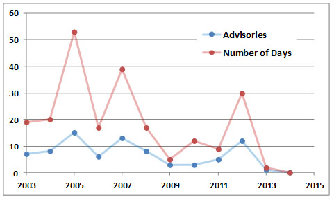
Because of the importance of smog as a stressor of urban Canadians, governments have initiated programs to monitor air pollutants and predict their concentrations so that “smog alerts” can be issued to the public. Environment Canada, in partnership with provincial and municipal governments, routinely issues advisories in smog-prone cities, usually on the day before a high level of ozone is predicted. Similarly, some provinces and municipalities have developed air-quality indices to provide daily advisories. The intent is to encourage people and industries to take actions to reduce air pollution and to avoid unnecessary exposure by staying inside buildings and by not engaging in outdoor exercise that involves deep breathing.
In 2005, Ontario experienced its worst-ever smog summer, with 53 days between June and September having air so polluted by ozone and other chemicals that it was considered a health hazard. The smog was caused by emissions from the many vehicles and other sources in that well-populated region, coupled with weather that was hotter and sunnier than normal (those conditions favour the photochemical formation of ozone), as well as LRTAP from other regions. It appears that this sort of health-threatening smog is well established in extensive, highly populated regions of southern Ontario and elsewhere in Canada.
Figure 16.4. History of smog advisories in Ontario. Source: Data from Ontario Ministry of the Environment (2014).
Case Studies of Ecological Damage
In this section we examine two case studies of ecological damage caused by air pollution. The first example describes “natural” air pollution at the Smoking Hills, a remote locality in the Arctic. The second examines ecological effects of emissions from large smelters near Sudbury, Ontario.
The Smoking Hills
The Smoking Hills are located in the Northwest Territories on the coast of the Beaufort Sea. At various places along the coast and nearby rivers, seams of bituminous shale occur as exposed strata in steep places were erosion is occurring. The shale contains pyritic sulphur, which becomes oxidized to sulphate when exposed to atmospheric oxygen through erosion of the cliffs. The oxidation produces heat (the reaction is exothermic), which under insulating conditions can increase the temperature enough to spontaneously ignite the bituminous materials. These smoulder and release SO2, which fumigates the nearby tundra. The first recorded sighting of the Smoking Hills was in 1826 by John Richardson, an explorer. However, the burns were long known to local Inuit and are likely thousands of years old.
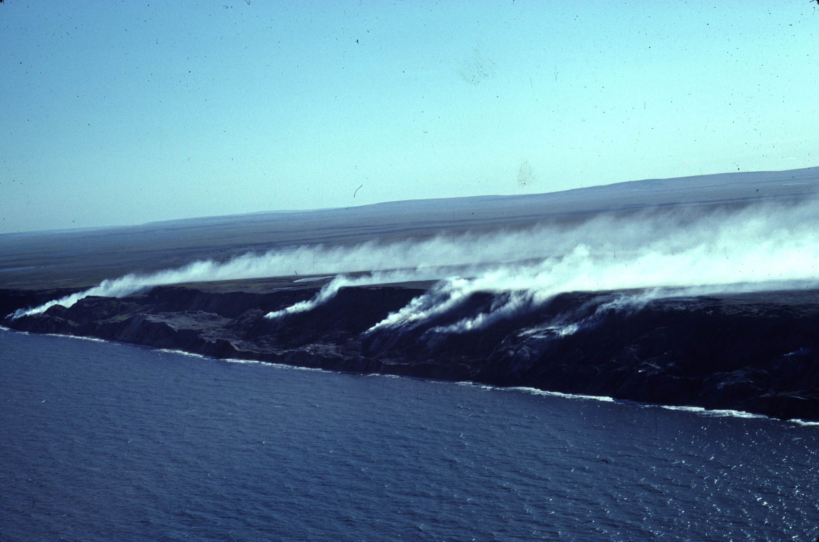
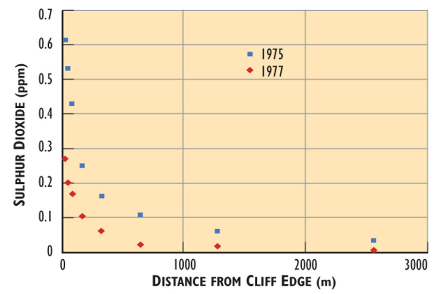
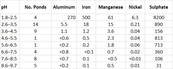
Winds at the Smoking Hills often blow the SO2-laden plumes (air masses) inland at ground level, such that they fumigate the tundra. The pollution is most intense at the edge of the cliff, where the plumes begin to spread inland. Concentrations of SO2 at the cliff edge are as high as 2 ppm, and then rapidly decrease inland in a more or less exponential manner (Figure 16.3). This gradient of air pollution occurs because the gases become progressively diluted in the ambient atmosphere with increasing distance from the points of emission.
The pollution by SO2 has severely acidified the soil. Acidic conditions in freshwater ponds reach pH 2 or less, compared with pH 8 or more outside the fumigation area (see In Detail 19.1 for an explanation of pH as a measure of acidity). The extreme acidification causes metals to become dissolved from minerals in soil and aquatic sediment (Table 16.4). High concentrations of solubilized metals are toxic to terrestrial and aquatic organisms. In addition, sulphate occurs in high concentrations in both soil and water. This is mostly a result of the dry deposition of SO2 from the atmosphere and its subsequent oxidation to SO42–within the ecosystem (see Chapter 19).
The high concentration of SO2 in the air and the acidity and soluble metals in soil and water result in the fumigated habitats being highly toxic to most plants, animals, and microorganisms. Close to the edge of the seacliff in fumigated areas, where the pollution is most intense, no vegetation grows at all – there is total ecological degradation. Farther inland, the pollution becomes less severe, and a few pollution-tolerant plants can grow. The most notable of these are arctic wormwood (Artemisia tilesii), polargrass (Arctagrostis latifolia), a lichen (Cladonia bellidiflora), and a moss (Pohlia nutans). These few tolerant plants have replaced the many species of unpolluted tundra, which includes arctic willow (Salix arctica), mountain avens (Dryas integrifolia), and more than 70 others (Freedman et al., 1990).
Pollution-tolerant species also occur in acidic ponds at the Smoking Hills. Even the most acidic ponds, which have a pH as low as 1.8, support at least six species of algae. These are extremely tolerant of acidity and dissolved metals and are not found in non-acidic waterbodies. In contrast to the acidic ponds, the unpolluted ponds are alkaline, with pH greater than 8, and they support rich algal communities of more than 90 species. A few acid-tolerant invertebrates also occur in acidic ponds (but only at pH greater than 2.8), including a crustacean (Brachionus urceolaris) and an insect midge (Chironomus riparius). The invertebrate fauna of non-acidic ponds is much richer in species and more productive (Havas and Hutchinson, 1983).
The most important lesson to be learned from the Smoking Hills is that “natural” pollution can cause ecological damage that is as intense as that associated with anthropogenic emissions. Clearly, SO2 can damage ecosystems regardless of the source of the pollution. In addition, the natural pollution at the Smoking Hills has stressed ecosystems for a long time – at least thousands of years – and the ecological effects have likely reached a steady-state condition. The study of the Smoking Hills provides some understanding of the long-term effects of severe air pollution:
- it causes a simplification of biodiversity and ecosystems to occur
- productivity and nutrient cycling are impaired
- unusual communities of pollution-tolerant species develop
Metal Smelters near Sudbury
In 1883, while blasting through bedrock during construction of the Canadian Pacific Railroad, a worker with some knowledge of prospecting discovered a rich body of metal-bearing ore in the vicinity of Sudbury, Ontario. The principal metals in the ore are nickel and copper. However, valuable quantities of iron, cobalt, gold, silver, and other metals are also produced from the mines, as are sulphur and selenium.
One of the world’s largest industrial complexes has been developed to mine and process the rich ore bodies near Sudbury. The facilities have included underground mines, an open-pit mine, ore-processing mills with tailings-disposal areas, smelters, metal refineries, sulphuric-acid plants, and various other installations. The industrial activities around Sudbury provide a key economic base for a regional population of more than 160-thousand people.
The metals in the Sudbury ore occur as sulphide minerals, meaning they are combined with sulphur in compounds such as nickel sulphide and iron sulphide. Consequently, an important step in processing the ore is to roast the material at a high temperature in the presence of oxygen, which converts the sulphides into gaseous SO2. The roasting increases the concentration of valuable metals in the residual material, which can then be smelted and refined into pure metals (see Figure 13.1).
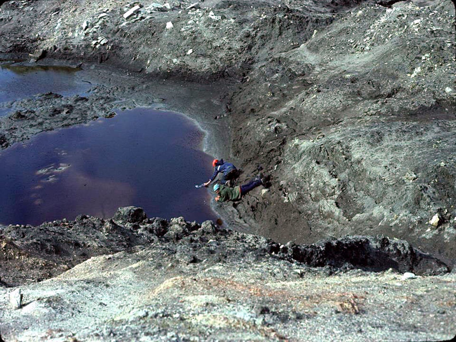
The large-scale roasting and smelting in the Sudbury area have resulted in huge emissions of SO2 and metal-containing particulates to the atmosphere, causing severe pollution and ecological damage. Until 1928, the roasting was conducted in huge open pits known as roast beds, which consisted of a layer of locally harvested cordwood over-heaped with sulphide ore. The wood was ignited, and the heat kindled the metal sulphides, releasing additional thermal energy because the oxidation is an exothermic reaction. The roast bed became hot enough to support a self-sustaining combustion of the ore, which would burn and smoulder for several months, after which the reactions were quenched with water. When the nickel and copper concentrates had cooled, they were collected and shipped to a refinery for further processing.
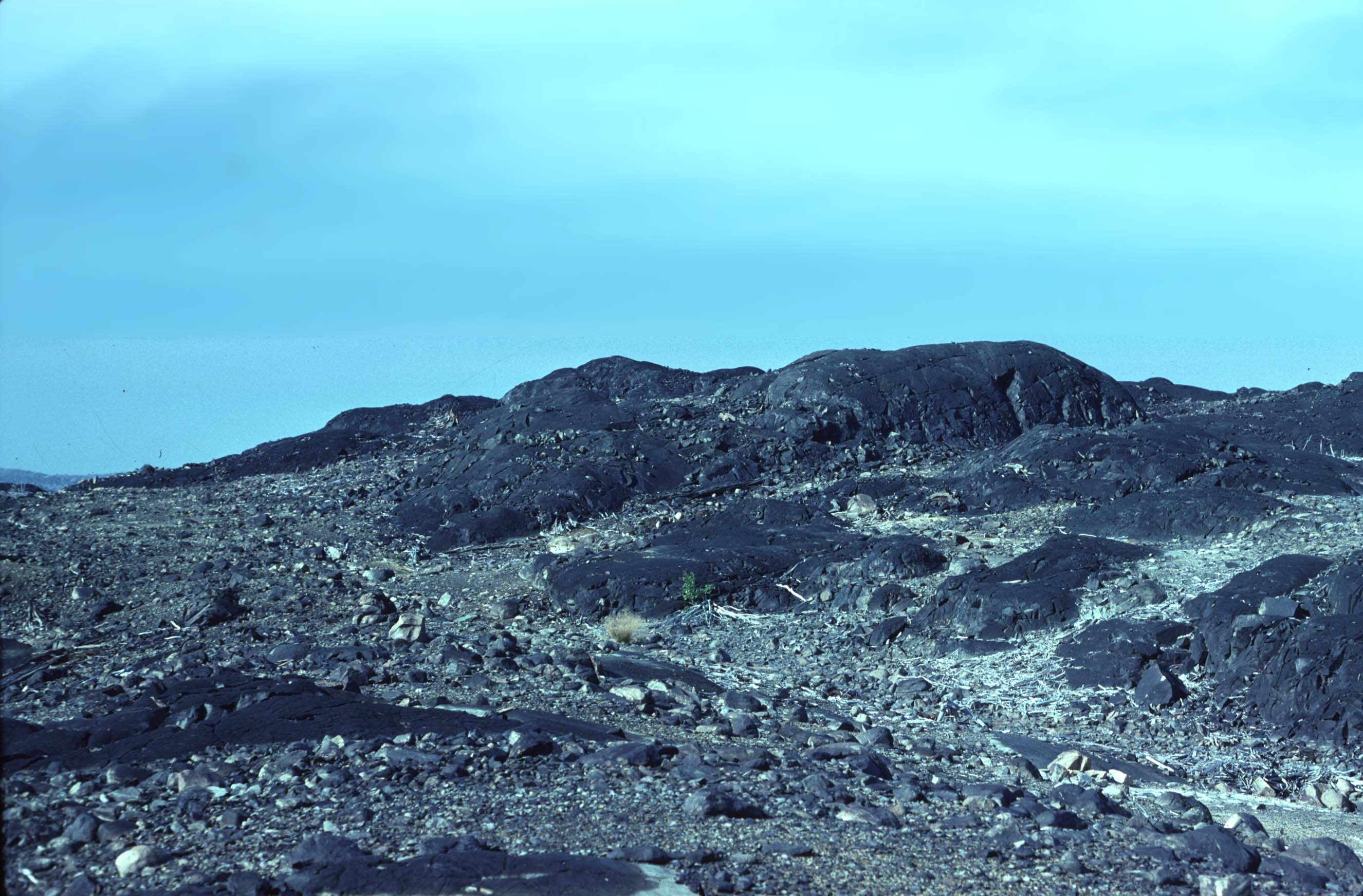
As is evident in the accompanying images, this crude roasting process resulted in intense ground-level fumigation of the landscape with toxic SO2, acidic mist, and metallic particulates. The pollution devastated ecosystems near the roast beds. The denuding of terrestrial habitats resulted in massive erosion of soil from slopes, exposing the bedrock, which became pitted and blackened by reaction with the sulphurous fumes.
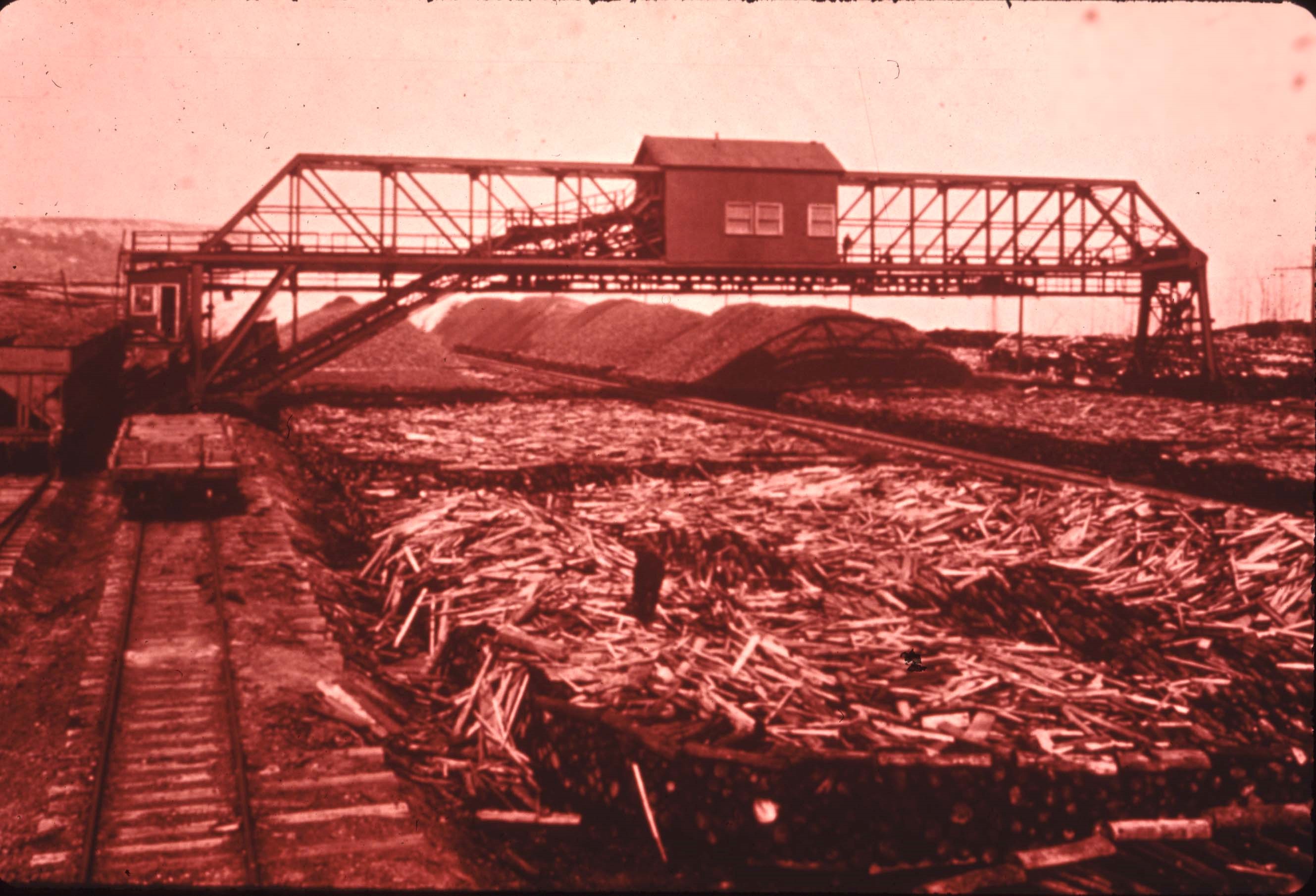
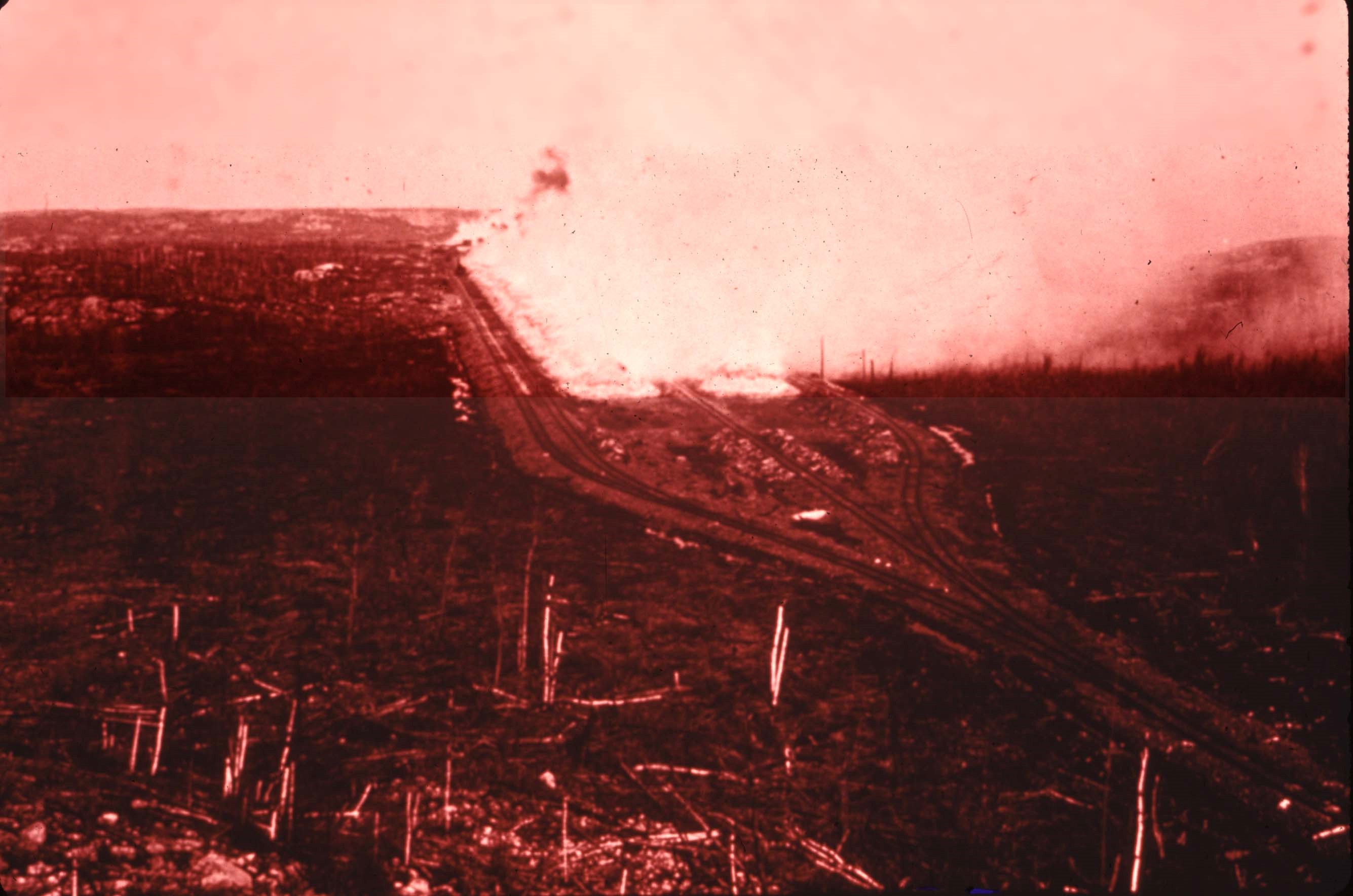
The 30 roast beds that operated in the Sudbury region emitted about 270-thousand tonnes per year of SO2 plus huge but undocumented amounts of metallic particulates. These early ground-level emissions caused the worst of the ecological damage in the Sudbury area.
In 1928, the government of Ontario prohibited any further use of roast beds. All roasting was then conducted at smelters located at Coniston, Copper Cliff, and Falconbridge, all in the vicinity of Sudbury. A smelter is a huge facility that contains roasting chambers within a building. Most of their emissions of waste gases and particulates are vented high into the atmosphere through a smokestack, which allows the pollutants to be dispersed and greatly reduces the severity of local ground-level pollution.
The largest smelter was built at Copper Cliff in 1929. Initially it had a single smokestack, with two others added in 1936. In 1972, the three stacks were replaced with a single 381-m “superstack” (at the time, the world’s tallest chimney, but now the second-tallest). At the same time, the Coniston smelter was closed and its production shifted to Copper Cliff. The Falconbridge smelter, with smokestacks of 93 m and 140 m, is owned by another company. The commissioning of the superstack in 1972 allowed pollutants to be vented high enough into the atmosphere to make ground-level fumigations infrequent events. This resulted in a great improvement of air quality in the Sudbury area. Tall smokestacks facilitate the dispersion and mixing of emissions into ambient air. This is sometimes referred to as the “dilution solution to pollution.”
Because the superstack is so tall, its emissions are well dispersed into the regional atmosphere. Little of the vented SO2 is deposited locally, a fact reflected by the relatively good air quality in the region since 1972. In fact, studies have indicated that only about 1% of the SO2 emissions are deposited within 40 km of the superstack. This means that 99% of the SO2 is exported over a longer distance, which avoids local damage but contributes to the acidification of precipitation over a large region (see Chapter 19). The plume from the superstack can be detected chemically at distances 150 km or more away.
The emissions of pollutants have also been reduced by other methods. Devices such as electrostatic precipitators are used to recover metal-containing dusts from the smelter flue-gases, while SO2emissions have been reduced by installing wet scrubbers, building sulphuric-acid plants, and constructing a facility to separate iron sulphides from the more valuable minerals of nickel and copper.
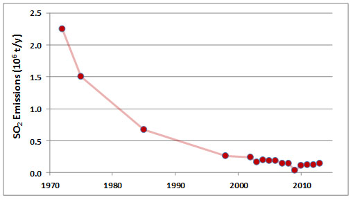
Emissions of SO2 in the Sudbury area peaked during 1960-1972, when discharges from the three smelters averaged about 2.25 million tonnes per year. At that time, Sudbury was the world’s largest source of anthropogenic SO2 emissions, responsible for about 4% of global releases. Emissions of SO2from the smelters have decreased greatly since that time, to about 0.14 x 10⁶ t/y during 2006-2013 (Figure 16.4; Environment Canada, 2014). The decreases are due mainly to expensive investments in pollution abatement technologies, including equipment for flue-gas desulphurization. Although greatly diminished, the emissions of SO2 remain large.
The post-superstack air quality in the Sudbury region represents a great improvement over the sulphurous past. Toxic fumigations with SO2, acidic mists, and metallic particulates were much more frequent and intense when roast beds were in use, as well as prior to 1972 when the smelters had shorter stacks and little pollution-abatement technology. Almost all of the worst of the ecological damage in the region resulted from the earlier emissions of pollutants. Other disturbances added to that damage, however, including the clear-cutting of forests to provide fuel for roast beds and the starting of wildfires by prospectors and by sparks from steam-powered railroad engines. The modern emissions of SO2 and other pollutants in the Sudbury region, while still large, are well dispersed and only infrequently cause acute biological damage. In fact, a substantial ecological recovery has occurred since the superstack was commissioned in 1972.
Large areas of land and surface water in the Sudbury region were severely damaged by pollution from the roast beds and smelters. The smelters are large, point-sources of emissions, so the severity of ecological damage decreased rapidly with an increasing distance away. Over the years, ecologists have documented vegetation damage in the area. In 1970, about 100 km2 of land around the smelters was characterized as “severely barren” and another 360 km2 had “impoverished” vegetation, including a lack of conifers in the forest (Watson and Richardson, 1972). White pine (Pinus strobus), an economically important tree, is sensitive to air pollution and it showed diagnostic SO2-injuries over an area of about 6,400 km2.
Pollution was especially damaging around Copper Cliff, the location of the largest smelter. The most degraded habitats occur within several kilometres of this facility and support almost no forest. Hills and slopes in this zone are extensively denuded of vegetation, their soil is eroded, and the exposed bedrock has been blackened by reaction with acidic fumigations. Only a few plant species that have evolved pollution-tolerant populations grow in this area, including several species of grasses, other herbaceous plants, and stunted, shrub-sized plants of some trees (see also Chapter 18).
The intensity of pollution-related stress rapidly lessens at greater distances from the smelters (there is a spatial gradient), and damage to vegetation is correspondingly less intense. About 3-8 km from the Copper Cliff smelter, remnants of forest survive where the local topography provided a degree of shelter from the pollution. However, denuded and blackened hilltops are still common in this patchily vegetated zone. Trees in the remnant stands are stunted, with many dead branches and other injuries. The trees include relatively pollution-tolerant species such as red maple (Acer rubium), white birch (Betula papyrifera), red oak (Quercus rubra), trembling aspen (Populus tremuloides), and large-toothed aspen (P. grandidentata). The forest cover beyond 8 km is almost continuous, but the biomass and biodiversity of the stands are impoverished. Beyond 20-30 km from the smelters, the forests are little affected by pollution and mixed stands of conifer and hardwood trees occur, as is typical of the region (Freedman and Hutchinson, 1980).
Lakes close to the Sudbury smelters were also severely degraded by atmospheric pollution. More than 7-thousand waterbodies in the region were acidified by the deposition of SO2 and contain elevated concentrations of toxic nickel, copper, and other metals. The polluted water bodies contain species-poor communities of tolerant algae, plants, and zooplankton. They lack fish, mostly because of their acidity.
However, great improvements in ground-level air quality since the building of the superstack in 1972 have resulted in dramatic ecological recoveries in the Sudbury area. Where eroded soil collected in moist basins, wet meadows developed. These are dominated by hairgrass (Deschampsia caespitosa), whose local populations are genetically tolerant to toxic nickel and copper in the soil (see Chapter 18). Other plants have also benefited from the reduction in air pollution, although their recovery is still impeded by residual soil toxicity associated with acidification and metals.
Lakes are also recovering in the region. In a set of 44 lakes that were monitored since 1981, including 28 that were highly acidified (to pH 5.0 or less), only 6 were that acidic in 2004 and 14 had recovered to pH 6.0, a level that would support most of the aquatic biota typical of the region (Keller et al., 2007). The concentrations of smelter-related metals, such as copper and nickel, are also much less, although still elevated compared with background conditions. In 1972, the pH of Baby Lake was 4.0-4.2, and it was almost devoid of algae and had no invertebrates or fish (Havas et al., 1995). However, by 1985 it had recovered to pH 6.8 and by 1995 to pH 7.2, and metals also decreased in concentration. Those improvements in water quality allowed the lake to be colonized by a diversity of phytoplankton, aquatic plants, invertebrates, and even small fishes.
Since the early 1970s, the ecological recovery of some degraded areas has been assisted by various management practices. The most important of these has been the liming of soil to reduce the acidity and thereby alleviate toxicity associated with metals. Also important have been the sowing of grasses and other plants that are known to be tolerant to the toxic conditions, the addition of fertilizer, and the planting of tree seedlings. Similar efforts in lakes have involved liming to reduce their acidity and metal toxicity, which has promoted the recovery of the biota. These efforts of reclamation, along with the natural regeneration that has occurred because of the greatly decreased pollution since the superstack was built, have helped to greatly improve degraded habitats in the Sudbury region.
The case of Sudbury is perhaps the world’s best-documented example of ecological damage caused by toxic gases and metals emitted from smelters. There are, however, additional examples of this sort of damage around other smelters in Canada, affecting smaller areas, such as the smelters at Flin Flon, MB, Rouyn-Noranda, QC, Trail, BC, and Yellowknife, NT.
These smelters are all large, point-sources of emissions of pollutants into the atmosphere. All developed pronounced spatial gradients in the intensity of pollution, which decreased exponentially with increasing distance from the source of emissions until the ambient condition is reached. The patterns of ecological damage track these spatial gradients of toxic stress.
Conclusions
Gaseous air pollutants, such as sulphur dioxide and nitric oxide, are emitted from a variety of sources, which range from large power plants and smelters to individual automobiles and home furnaces. In contrast, secondary pollutants such as ozone are not emitted but are formed in the atmosphere by photochemical reactions involving sunlight and emitted oxides of nitrogen and hydrocarbons. If their concentrations are high enough, gaseous pollutants (often in combination with particulates) can be a risk to human health, and they may cause severe ecological damage. Because these risks are now well known, many governments have taken steps to reduce the emissions of the most important air pollutants. This is particularly the case for relatively developed countries, such as Canada. Although the emissions of air pollutants in wealthy countries remain large, they are generally stabilizing or even decreasing. However, in rapidly growing economies, such as China and India, hasty and poorly controlled industrialization is resulting in rapidly worsening air pollution.
Questions for Review
- Compare the natural and anthropogenic emissions of sulphur and nitrogen compounds. Why do the sources of emission vary between regions and countries?
- Why are high concentrations of ozone in the lower atmosphere considered an environmental problem? Why does this differ from the stratosphere, where too little ozone is a problem?
- Explain are the differences between primary and secondary air pollutants? Give examples of each.
- Why has air pollution decreased so much in the Sudbury region, and what have been the ecological responses to this environmental improvement?
Questions for Discussion
- Compare, in broad terms, the patterns of ecological damage caused by “natural” pollution at the Smoking Hills with those caused by smelters near Sudbury. Why is it useful to study the ecological effects of natural pollution?
- Existing clean-air technologies could be used to greatly reduce the emissions of air pollutants everywhere. Considering the damage that pollutants cause to human health, ecosystems, and other values, why are these technologies not being used more extensively? Consider factors associated with economics, politics, scientific uncertainty about pollution damage, and the benefits of having cleaner air. Contrast the lack of action with the successes achieved in controlling the emissions of ozone-depleting substances through the Montreal Protocol.
- Epidemiological (statistical) research suggests that human health may be affected by ambient levels of air pollutants in urban areas, particularly through increased incidences of respiratory diseases, such as asthma. However, the statistical data are rather weak, and only a relatively small proportion of the urban population appears to be affected. What are some issues that decision makers must consider when deliberating about additional controls on the release of air pollutants in urban areas?
- Like most other smelters built during the twentieth century, the ones at Sudbury caused obvious damage to ecosystems and human health. Why were those large industrial facilities not shut down or better controlled by the governments of the day? Today, new smelters are being built in Canada and in other countries. Are there risks of those industrial facilities repeating the mistakes of the past?
Exploring Issues
- You have been asked to assess the potential ecological effects of building a new metal smelter in a region that is now wilderness. The smelter will emit sulphur dioxide to the atmosphere. Based on what you know about pollution damage at the Smoking Hills, around Sudbury, and at other smelters, what would be the most important considerations to incorporate into the environmental impact assessment? Focus on the potential effects on terrestrial and aquatic ecosystems.
References Cited and Further Reading
Anderson, S.O. and K.M. Sarma. 2005. Protecting the Ozone Layer: The United Nations History. Earthscan Publications, London, UK.
Ayres, J. and R.L. Maynard. 2006. Air Pollution and Health. World Scientific Publishing Company.
Barker, J.R. and D.T. Tingey. 1992. Air Pollution Effects on Biodiversity. Van Nostrand Reinhold, New York, NY.
Brimblecombe, P. 1996. Air Composition and Chemistry. 2nd ed. Cambridge University Press, Cambridge, UK.
Brimblecombe, P. 2005. The Effects of Air Pollution on the Built Environment. Imperial College Press, London, UK.
Canadian Council of Ministers of the Environment (CCME). 2014. Canadian Environmental Quality Guidelines. CCME. Winnipeg, MB. http://www.ccme.ca/en/resources/canadian_environmental_quality_guidelines/index.html Accessed January, 2015.
Environment Canada. 1999. Ground-Level Ozone: Occurrence and Transport in Eastern North America. Hackensack, NJ.
Environment Canada. 2013. Canadian Ambient Air Quality Standards. http://www.ec.gc.ca/default.asp?lang=En&n=56D4043B-1&news=A4B2C28A-2DFB-4BF4-8777-ADF29B4360BD Accessed January 2015.
Environment Canada. 2014. National Pollutant Release Inventory and Air Pollutant Emission Summaries and Trends. Environment Canada, Ottawa, ON. http://www.ec.gc.ca/inrp-npri/default.asp?lang=en&n=0EC58C98-1#Emission_Summaries Accessed January 2015.
Environmental Protection Agency (U.S.). 2014. Air Trends. US EPA, Research Triangle Park, NC. www.epa.gov/airtrends/ Accessed January, 2014.
Freedman, B. 1995. Environmental Ecology. 2nd ed. Academic Press, San Diego, CA. Freedman, B. and T.C. Hutchinson. 1980. Long-term effects of smelter pollution at Sudbury, Ontario, on forest community composition. Canadian Journal of Botany, 58: 2123-2140.
Freedman, B., V. Zobens, and T.C. Hutchinson. 1990. Intense, natural pollution affects arctic tundra vegetation at the Smoking Hills, Canada. Ecology, 71: 492-503.
Gizyn, W. 1980. The Chemistry and Environmental Impact of the Bituminous Shale Fires at the Smoking Hills, NWT. M.Sc. Thesis, University of Toronto, Toronto, ON.
Gunn, J.M. (ed.). 1995. Restoration and Recovery of an Industrial Region: Progress in Restoring the Smelter-Damaged Landscape near Sudbury, Canada. Springer, New York, NY.
Havas, M. and T.C. Hutchinson. 1983. The Smoking Hills: Natural acidification of an aquatic ecosystem. Nature, 301: 23-–27.
Havas, M., D.G. Woodfine, P. Lutz, K. Yung, H.H. MacIsaac, and T.C. Hutchinson. 1995. Biological recovery of two previously acidified, metal-contaminated lakes near Sudbury Ontario, Canada. Water, Air and Soil Pollution, 85: 791-796.
Hemond, H.F. and E.J. Fechner. 2014. Chemical Fate and Transport in the Environment. 3rd ed. Academic Press, San Diego, CA.
Hester, R.E. and R.M. Harrison. 1998. Air Pollution and Health. Royal Society of Chemistry, Cambridge, UK.
Holgate, S.T., J.M. Samet, R.L. Maynard, and H.S. Koren (eds.). 1999. Air Pollution and Health. Academic Press, San Diego, CA.
Keller, W., N.D. Yan, J.M. Gunn, and J. Heneberry. 2007. Recovery of acidified lakes: Lessons From Sudbury, Ontario, Canada. Water, Air and Soil Pollution: Focus, 7: 317-322. Maynard, R.L. and P. Brimblecombe (eds.). 2001. The Urban Atmosphere and Its Effects. World Scientific Publishing Company, Hackensack, NJ.
National Weather Service (U.S.). 2015. Meteorological Conditions and Ozone in the Polar Stratosphere. NWS, Washington, DC. Accessed January, 2015. www.cpc.ncep.noaa.gov/products/stratosphere/polar/polar.shtml
Netherlands Environmental Assessment Agency (NEAA). 2015. Emission Database for Global Environmental Research (EDGAR). NEAA. The Hague, The Netherlands. http://themasites.pbl.nl/tridion/en/themasites/edgar/emission_data/edgar_32ft2000/index-2.html Accessed January, 2015.
Ontario Medical Association (OMA). 2015. Smog/Air Pollution. Resources. OMA, Toronto, ON. https://web.archive.org/web/20160914204453/https://www.oma.org/HealthPromotion/Smog/Pages/default.aspx .
Ontario Ministry of the Environment and Climate Change. 2014. Summary of Smog Advisories. OMECC, Toronto, ON. http://www.airqualityontario.com/press/smog_advisories.php Accessed January 2015.
Parson. E. 2003. Protecting the Ozone Layer: Science and Strategy. Oxford University Press, Oxford, UK.
Pepper, I.L., C.P. Gerba, and M.L. Brusseau (eds.). 2006. Pollution Science, 2nd ed. Academic Press, San Diego, CA.
Roberts, T.M. 1984. Effects of air pollutants in agriculture and forestry. Atmospheric Environment, 18: 629-652.
Seinfeld, J.H. and S.H. Pandis. 2006. Atmospheric Chemistry and Physics: From Air Pollution to Climate Change, 2nd ed. Wiley-Interscience, New York, NY.
Shriner, D.S. 1990. Responses of vegetation to atmospheric deposition and air pollution. In Acidic Deposition: State of Science and Technology. Vol. III. Terrestrial, Materials, Health, and Visibility Effects. Superintendent of Documents, U.S. Government Printing Office, Washington, DC.
Vallero, D. 2014. Fundamentals of Air Pollution, 5th ed. Academic Press, San Diego. Wark, K. Jr., C.F. Warner, and W.T. Davis. 1998. Air Pollution: Its Origin and Control. 3rd ed. Addison-Wesley, Menlo Park, CA.
Watson, W.Y. and D.H. Richardson. 1972. Appreciating the potential of a devastated land. Forestry Chronicle, 48: 312-315.
Winterhalder, E.K. 1978. A historical perspective of mining and reclamation in Sudbury. Proceedings, 3rd Annual Meeting, Canadian Land Reclamation Association. Guelph, ON.
Wise, W. 2001. Killer Smog: The World’s Worst Air Pollution Disaster. Author’s Guild, New York, NY.