
3.2: Determining a Distribution in the Absence of Data
- Page ID
- 30965

Often, parameter values for probability distributions used to model random quantities must be determined in the absence of data. There are many possible reasons for a lack of data. The simulation study may involve a proposed system. Thus, no data exists. The time and cost required to obtain and analyze data may be beyond the scope of the study. This could be especially true in the initial phase of a study where an initial model is to be built and initial alternatives analyzed in a short amount of time. The study team may not have access to the information system where the data resides.
The distribution functions commonly employed in the absence of data are presented. An illustration of how to select a particular distribution to model a random quantity in this case is given.
3.2.1 Distribution Functions Used in the Absence of Data
Most often system designers or other experts have a good understanding of the “average” value. Often, what they mean by “average” is really the most likely value or mode. In addition, they most often can supply reasonable estimates of the lower and upper bounds that is the minimum and maximum values. Thus, distribution functions must be used that have a lower and upper bound and whose parameters can be determined using no more information than a lower bound, upper bound, and mode.
First consider the distribution functions used to model operation times. The uniform distribution requires only two parameters, the minimum and the maximum. Only values in this range [min, max] are allowed. All values between the minimum and the maximum are equally likely. Normally, more information is available about an operation time such as the mode. However, if only the minimum and maximum are available the uniform distribution can be used.
Figure 3-1 provides a summary of the uniform distribution.
Figure 3-1: Summary of the Uniform Distribution
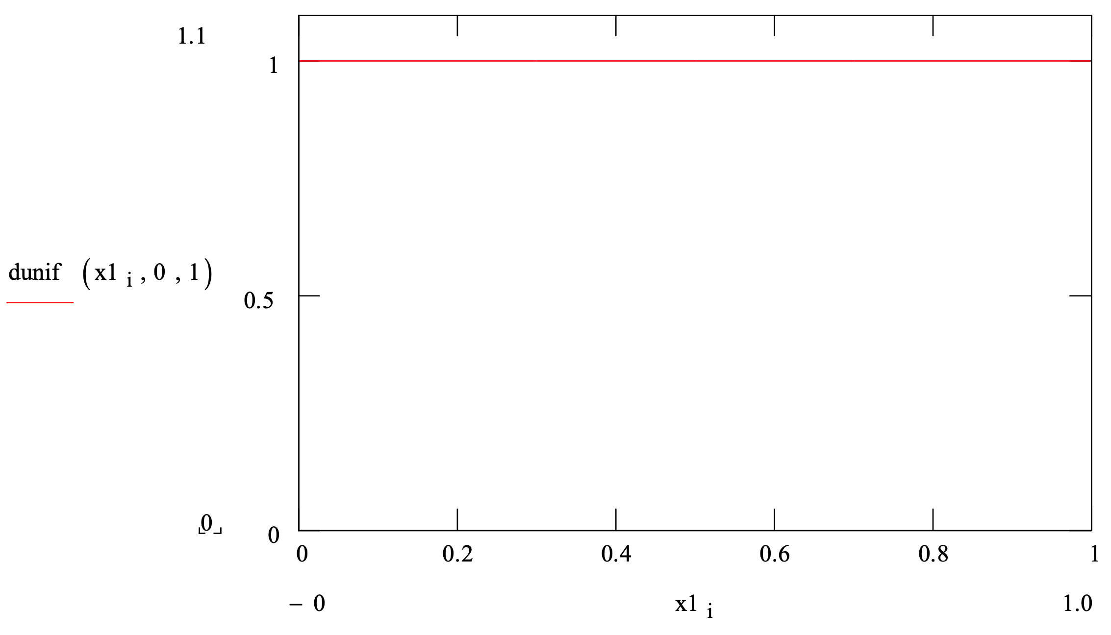
Density Function Illustration
| Parameters: | min(imum) and max(imum) |
| Range: | [min, max] |
| Mean: | \(\ \text { mean }=\frac{\min +\max }{2}\) |
| Variance: | \(\ \text { variance }=\frac{(\max -\min )^{2}}{12}\) |
| Density function: | \(\ f(x)=\frac{1}{\max -\min } ; \min \leq x \leq \max\) |
| Distribution function: | \(\ F(x)=\frac{x-\min }{\max -\min } ; \min \leq x \leq \max\) |
| Application: | In the absence of data, the uniform distribution is used to model a random quantity when only the minimum and maximum can be estimated. |
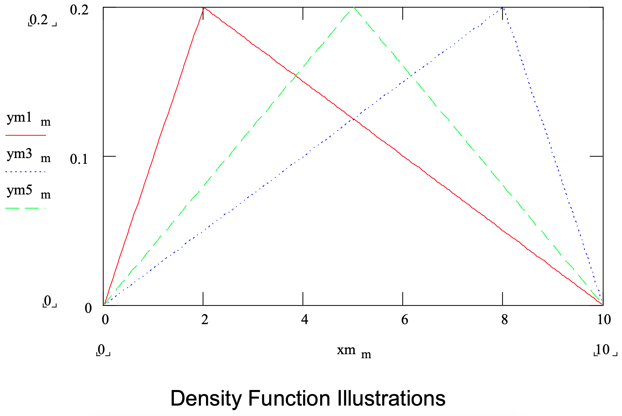
If the mode is available as well, the triangular distribution can be used. The minimum, maximum, and mode are the parameters of this distribution. Note that the mode can be closer to the minimum than the maximum so that the distribution is skewed to the right. Alternatively, the distribution can be skewed to the left so that the mode is closer to the maximum than the minimum. The distribution can be symmetric with the mode equidistant from the minimum and the maximum. These cases are illustrated in Figure 3-2 where a summary of the triangular distribution is given.
Figure 3-2: Summary of the Triangular Distribution
| Parameters: | min(imum), mode, and max(imum) |
| Range: | [min, max] |
| Mean: | \(\ \frac{min +mode +max }{3}\) |
| Variance: | \(\ \frac{min^2 +mode^2 +max^2 -min * mode \ -min *max -mode * max }{18}\) |
| Density function: | \(\ f(x)=\left\{\begin{array}{cc} \frac{2^{*}(\mathbf{x}-\mathbf{m i n})}{(\max -\min ) *(\operatorname{mode}-\min )} ; \min \leq \mathbf{x} \leq \operatorname{mode} \\ \frac{2^{*}(\max -\mathbf{x})}{(\max -\min ) *(\max -\operatorname{mode})} ; \operatorname{mode} <\mathbf{x}<\max \end{array}\right\}\) |
| Distribution function: | \(\ F(x)=\left\{\begin{array}{lc} \frac{(x-m i n)^{2}}{(\max -m i n) *(m o d e-m i n)} ; \min \leq x \leq \text { mode } \\ 1-\frac{(\max -x)^{2}}{(\max -m i n) *(\max -m o d e)} ; \text { mode }<x<\max . \end{array}\right\}\) |
| Application: | In the absence of data, the triangular distribution is used to model a random quantity when the most likely value as well as the minimum and maximum can be estimated. |
The beta distribution provides another alternative for modeling an operation time in the absence of data. The triangular distribution density function is composed of two straight lines. The beta distribution density function is a smooth curve. However, the beta distribution requires more information and computation to use than does the triangular distribution. In addition, the beta distribution is defined on the range [0,1] but can be easily shifted and scaled to the range [min, max] using min + (max-min)*X, where X is a beta distributed random variable in the range [0, 1]. Thus, as did the uniform and triangular distributions, the beta distribution can be used for values in the range [min, max].
Using the beta distribution requires values for both the mode and the mean. Subjective estimates of both of these quantities can be obtained. However, it is usually easier to obtain an estimate of the mode than the mean. In this case, the mean can be estimated from the other three parameters using equation 3-1.
\(\ \begin{align}mean = \frac{min + mode + max}{3}\tag{3-1}\end{align}\)
Pritsker (1977) gives an alternative equation that is similar to equation 3-2 except the mode is multiplied by 4 and the denominator is therefore 6.
The two parameters of the beta distribution are \(\ \alpha_{1}\) and \(\ \alpha_{2}\). These are computed from the minimum, maximum, mode, and mean using equations 3-2 and 3-3.
\(\ \begin{align}\alpha_{1}=\frac{(\mathrm{mean}-\min ) *(2 * \mathrm{mode}-\min -\mathrm{max})}{(\mathrm{mode}-\operatorname{mean}) *(\max -\min )}\tag{3-2}\end{align}\)
\(\ \begin{align}\alpha_{2}=\frac{(\max -\operatorname{mean}) * \alpha_{1}}{\operatorname{mean}-\min }\tag{3-3}\end{align}\)
Most often for operation times, \(\ \alpha_{1}\) 1 and \(\ \alpha_{2}\) > 1. Like the triangular distribution, the beta distribution can be skewed to the right \(\ \alpha_{1}<\alpha_{2}\), skewed to the right, \(\ \alpha_{1}>\alpha_{2}\), or symmetric, \(\ \alpha_{1}=\alpha_{2}\). A summary of these and other characteristics of the beta distribution is given in Figure 3-3.
Next, consider modeling the time between entity arrivals. In the absence of data, all that may be known is the average number of entities expected to arrive in a given time interval. The following assumptions are usually reasonable when no data are available.
- The entities arrive one at a time.
- The mean time between arrivals is the same over all simulation time.
- The numbers of customers arriving in disjoint time intervals are independent.
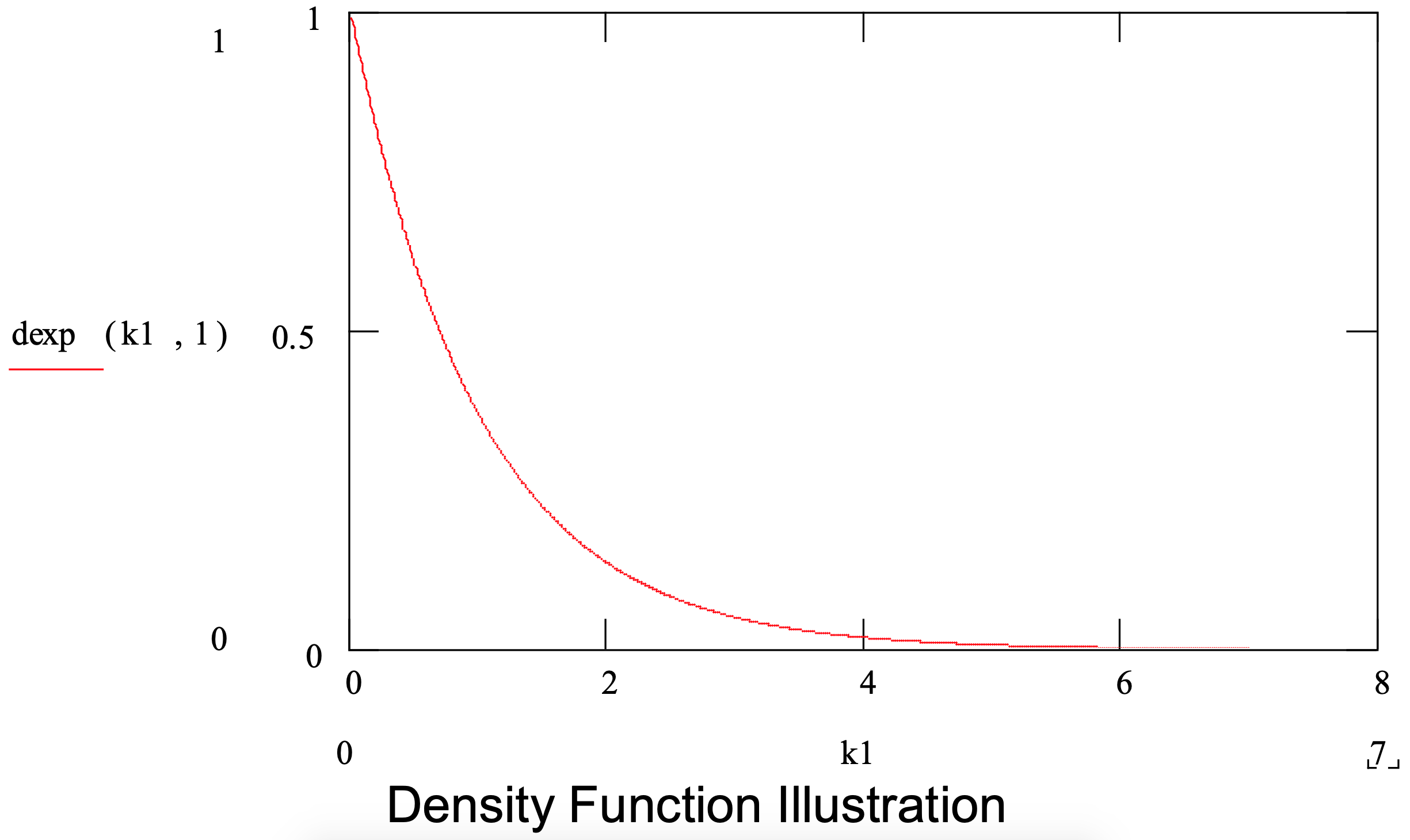
All of this leads to using the exponential distribution to model the times between arrivals. The exponential has one parameter, its mean. The variance is equal to the mean squared. Thus, the mean is equal to the mean time between arrivals or the time interval of interest divided by an estimate of the number of arrivals in that interval.
Using the exponential distribution in this case can be considered to be a conservative approach as discussed by Hopp and Spearman (2007). These authors refer to a system with exponentially distributed times between arrivals and service times as the practical worst case system. This term is used to express the belief that any system with worse performance is in critical need of improvement. In the absence of data to the contrary, assuming that arrivals to a system under study are no worse than in the practical worse case seems safe.
Figure 3-4 summarizes the exponential distribution.
Figure 3-3: Summary of the Beta Distribution
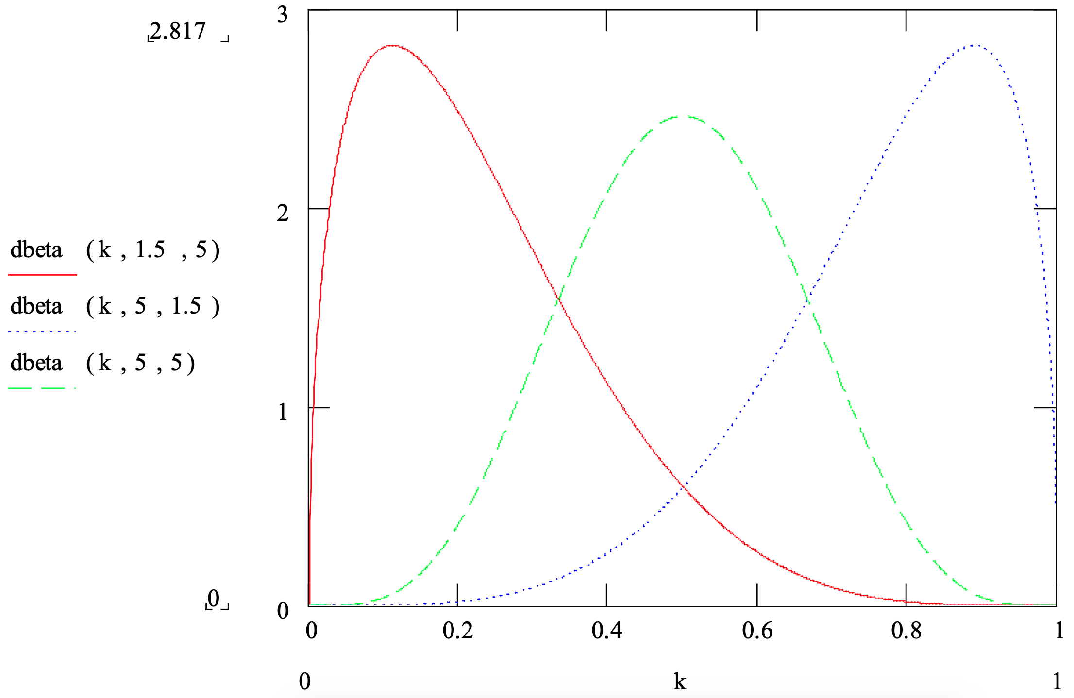 Density Function Illustrations
| Parameters: | min(imum), mode, mean, and max(imum) |
| Range: | [min, max] |
| Mean: | \(\ \frac{\alpha_{1}}{\alpha_{1}+\alpha_{2}}\) |
| Variance: | \(\ \frac{\alpha_{1}\ {*}\ \alpha_{2}}{\left(\alpha_{1}+\alpha_{2}\right)^{2} *\left(\alpha_{1}+\alpha_{2}+1\right)}\) |
| Density function: | \(\ f(x)=\frac{x^{\alpha_{1}-1}(1-x)^{\alpha_{2}-1}}{B\left(\alpha_{1}, \alpha_{2}\right)} ; 0<x<1\) |
| The denominator is the beta function. | |
| Distribution function: | No closed form. |
| Application: | In the absence of data, the beta distribution is used to model a random quantity when the minimum, mode, and maximum can be estimated. If available, an estimate of the mean can be used as well or the mean can be computed from the minimum, mode, and maximum. Traditionally, the beta distribution has been used to model the time to complete a project task. When data are available, the beta can be used to model the fraction, 0 to 100%, of something that has a certain characteristic such as the fraction of scrap in a batch. |
Figure 3-4: Summary of the Exponential Distribution
| Parameter: | mean |
| Range: | [0, \(\ \infty\)) |
| Mean: | given parameter |
| Variance: | mean2 |
| Densityfunction: | \(\ f(x)=\frac{1}{\text { mean }} e^{-x / \text {mean}} ; x \geq 0\) |
| Distributionfunction: | \(\ F(x)=1-e^{-x / \text {mean}} ; x \geq 0\) |
| Application: | The exponential is used to model quantities with high variability such as entity inter-arrival times and the time between equipment failures as well as operation times with high variability. In the absence of data, the exponential distribution is used to model a random quantity characterized only by the mean. |
3.2.2 Selecting Probability Distributions in the Absence of Data – An Illustration
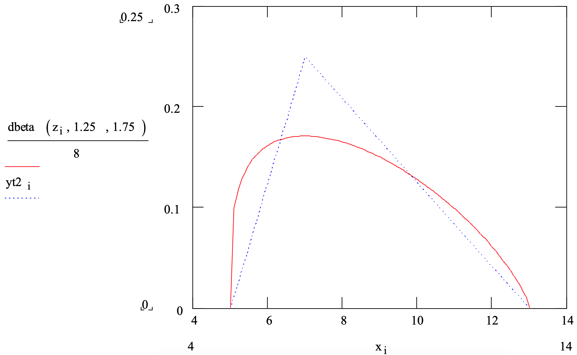
Consider the operation time for a single workstation. Suppose the estimates of a mode of 7 seconds, a minimum of 5 seconds, and a maximum of 13 seconds were accepted by the project team. Either of two distributions could be selected.
- A triangular with the given parameter values and having a squared coefficient of variation1 of 0.042.
- A beta distribution with parameter values \(\ \alpha_{1}\) = 1.25 and \(\ \alpha_{2}\) = 1.75 and a squared coefficient of variation of 0.061 where equations 3-3 and 3-4 were use to compute \(\ \alpha_{1}\) and \(\ \alpha_{2}\).
The mean of the beta distribution was estimated as the arithmetic average of the minimum, maximum, and mode. Thus, the mean of the triangular distribution and of the beta distribution are the same.
Note that the choice of distribution could significantly affect the simulation results since the squared coefficient of variation of the beta distribution is about 150% of that of the triangular distribution. This means the average time in the buffer at workstation A will likely be longer if the beta distribution is used instead of the triangular. This idea will be discussed further in Chapter 5.
Figure 3-5 shows the density functions of these two distributions.
Figure 3-5: Probability Density Functions of the Triangular (5, 7, 13) and Beta (1.25, 1.75)
A word of caution is in order. If there is no compelling reason to choose the triangular or the beta distribution then a conservative course of action would be to run the simulation first using one distribution and then the other. If there is no significant difference in the simulation results or at least in the conclusions of the study, then no further action is needed. If the difference in the results is significant, both operationally and statistically, further information and data about the random quantity being model should be collected and studied.
1 The coefficient of variation is the standard deviation divided by the mean. The smaller this quantity the better.
Furthermore, it was estimated that there would be 14400 arrivals per 40-hour week to the two workstations in a series system. Thus, the average time between arrivals is 40 hours / 14400 arrivals = 10 seconds. The time between arrivals was modeled using an exponential distribution with mean 10 seconds.