3.3: Fitting a Distribution Function to Data

This section discusses the use of data in determining the distribution function to use to model a random quantity as well as values for the distribution parameters. Some common difficulties in obtaining and using data are discussed. The common distribution functions used in simulation models are given. Law (2007) provide an in depth discussion of this topic, including additional distribution functions. A software based procedure for using data in selecting a distribution function is presented.

3.3.1 Some Common Data Problems

It is easy to assume that data is plentiful and readily available in a corporate information system. However, this is often not the case. Some problems with obtaining and using data are discussed.

1. Data are available in the corporate information system but no one on the project team has permission to access the data.

   Typically, this problem is resolved by obtaining the necessary permission. However, it may not be possible to obtain this permission in a timely fashion. In this, case the procedures for determining a distribution function in the absence of data should be used at least initially until data can be obtained.

2. Data are available but must be transformed into values that measure the quantity of interest.

   For example, suppose the truck shipment time between a plant and a customer is of interest. The company information system records the following clock times for each truck trip: departure from the plant, arrival to the customer, departure from the customer, and arrival to the plant. The following values can be computed straightforwardly from this information for each truck trip: travel time from the plant to the customer, time delay at the customer, travel time from the customer to the plant.

   This example raises some other questions. Is the there any reason to believe that the travel time from the plant to the customer is different from the travel time from the customer to the plant? If not, the two sets of values could be combined and a single distribution could be determined from all the values. If there is a known reason that the travel times are different, the two data sets must be analyzed separately. Of course, a statistical analysis, such as the paired-t method discussed in chapter 4, could be used to assess whether any statistically significant difference in the mean travel times exists.

   What is the level of detail included in the model? It may be necessary to include all three times listed in the previous paragraph in the model. Alternatively, only the total round trip time, the difference between the departure from the plant and the arrival to the plant, could be included.

3. All the needed data is available, but only from multiple sources.

   Each of the multiple sources may measure quantities in different ways or at different times. Thus, data from different sources need to be made consistent with each other. This is discussed by Standridge, Pritkser, and Delcher (1978).

   For example, the amount of sales of a chemical product is measured in pounds of product in the sales information system and in volume of product in the shipping information system. The model must measure the amount of product in either pounds or volume. Suppose pounds were chosen. The data in the shipping information system could be used after dividing it by product density (pounds/gallon).

   Consider another example. A sales forecast is used to establish the average volume of demand for a product used in a model. The sales forecast for the product is a single value. A distribution of product demand is needed. A distribution is determined using historical sales data. The sales forecast is used as the mean of a distribution instead of the mean computed from historical data. This assumes that only the mean will change in the future. The other distribution parameters such as the variance as well as the particular distribution family, normal for example, will remain the same.

4. All data are “dirty”.

   It is tempting to assume that data from a computer information system can be used without further examination or processing. This is often not the case. Many data collection mechanisms do not take into account the anomalies that occur in day-to-day system operations.

   For example, an automated system records the volume of a liquid product produced each day. This production volume is modeled as a single random quantity. The recorded production volume for all days is greater than zero. However, on a few days it is two orders of magnitude less than the rest of the days. It was determined that these low volumes meant that the plant was down for the day. Thus, the production volume was modeled by a distribution function for the days that the plant was operating and zero for the remaining days. Each day in the simulation model, a random choice was made as to whether or not the plant was operating that day. The probability the plant was operating was estimated from the data set as percent of days operating / total number of days.

3.3.2 Distribution Functions Most Often Used in a Simulation Model

In this section, the distribution functions most often used in simulation models are presented. The typical use of each distribution is described. A summary of each distribution is given.

In section 3.2.1, distribution functions used in the absence of data were presented. The uniform and triangular distributions are typically only used in this case. The beta distribution is used as well. The beta is also useful modeling project task times.

In addition, the use of the exponential distribution to model the time between entity arrivals was discussed. Again, the conditions for using the exponential distribution are: there is one arrival at a time, the numbers of arrivals in disjoint time intervals are independent, and the average time until the next arrival doesn’t change over the simulation time period. In some cases, the latter assumption is not true. One way of handling this situation is illustrated in the application study concerning contact center management.

If the system exerts some control over arrivals, this information may be incorporated in the simulation. For example, arrivals of part blanks to a manufacturing system could occur each hour on the hour. The time between arrivals would be a constant 1 hour. Suppose that workers have noted that the blanks actually arrive anywhere between 5 minutes before and 5 minutes after the hour. Thus, the arrival process could be modeled as with a constant time between arrivals of 1 hour followed by a uniformly distributed delay of 0 to 10 minutes before processing begins.

Often it is important to include the failure of equipment in a simulation model. Models of the time till failure can be taken from reliability theory. The exponential distribution may also be used to model the time until the next equipment breakdown if the proper conditions are met: there is one breakdown at a time (for each piece of equipment), the number of breakdowns in disjoint time intervals are independent, and the average time until the next breakdown doesn’t change over the simulation time period.

Suppose either of the following is true:

1. The time from now till failure does depend on how long the equipment has been functioning.
2. Failure occurs when the first of many components or failure points fails.

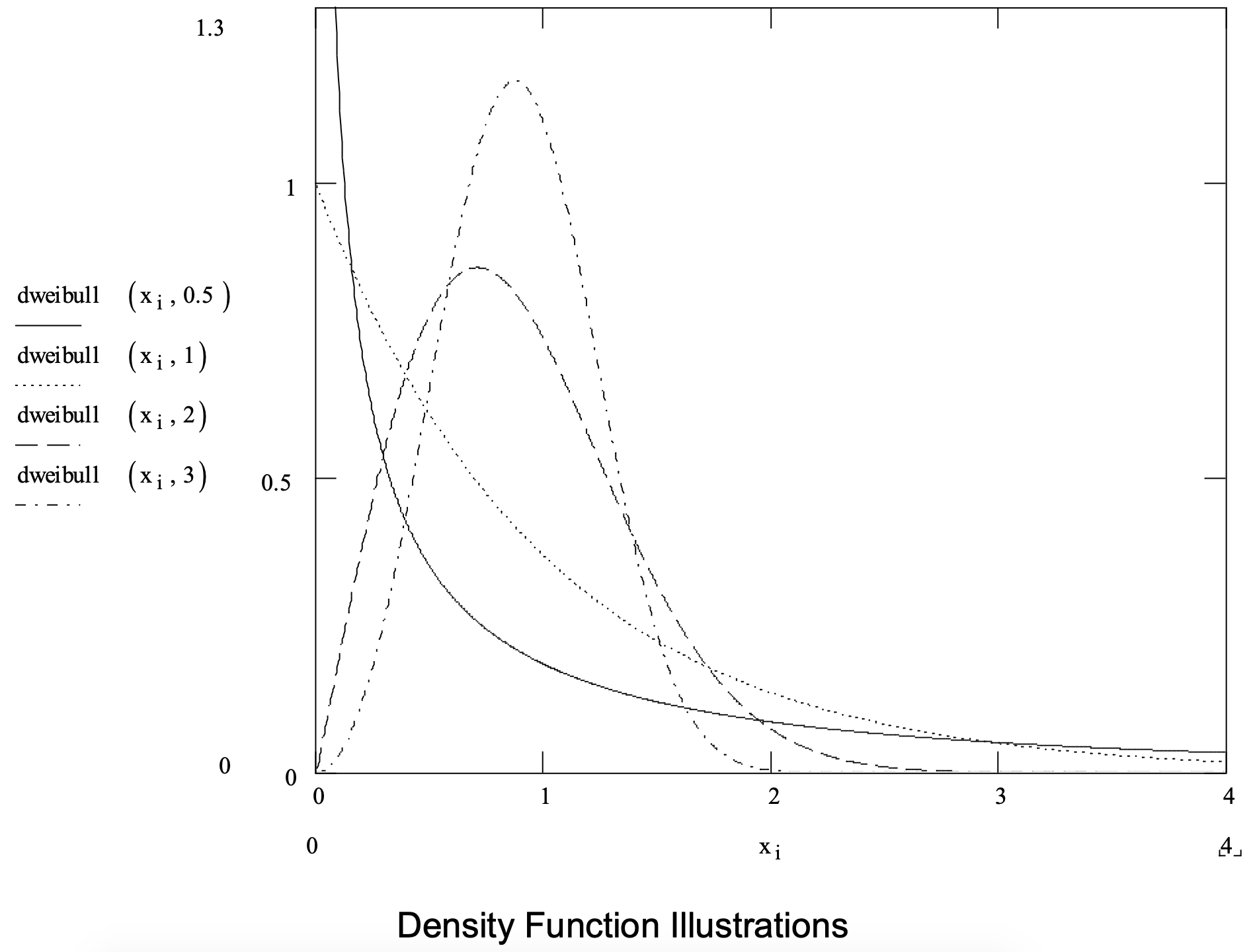
Under these conditions, the Weibull distribution is an appropriate model of the time between failures. The Weibull is also used to model operation times. A Weibull distribution has a lower bound of zero and extends to positive infinity.

A Weibull distribution has two parameters: a shape parameter \(\ \alpha\) > 0 and a scale parameter \(\ \beta\) > 0. Note that the exponential distribution is a special case of the Weibull distribution for \(\ \alpha\) = 1. A summary of the Weibull distribution is given in Figure 3-6.

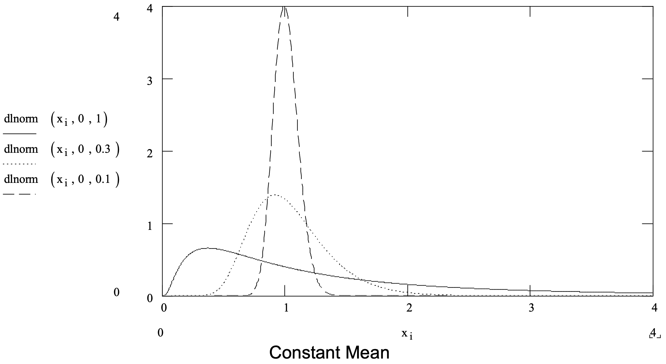
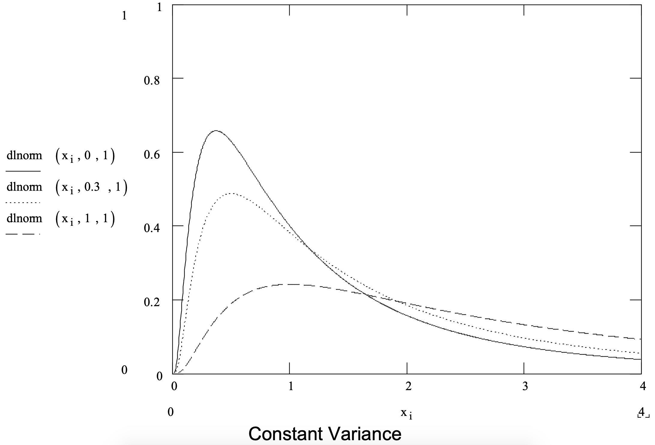
Suppose failure is due to a process of degradation and a mathematical requirement that the degradation at any point in time is a small random proportion of the degradation to that point in time is acceptable. In this case the lognormal distribution is appropriate. The lognormal has been successfully applied in modeling the time till failure in chemical processes and with some types of crack growth. It is also useful in modeling operation times.

The lognormal distribution can be thought of in the following way. If the random variable X follows the lognormal distribution then the random variable ln X follows the normal distribution. The lognormal distribution parameters are the mean and standard deviation of the normal distribution results from this operation. A lognormal distribution ranges from 0 to positive infinity. The lognormal distribution is summarized in Figure 3-7.

Consider operation, inspection, repair and transportation times. In modeling automated activities, these times may be constant. A constant time also could be appropriate if a standard time were assigned to a task. If human effort is involved, some variability usually should be included and thus a distribution function should be employed.

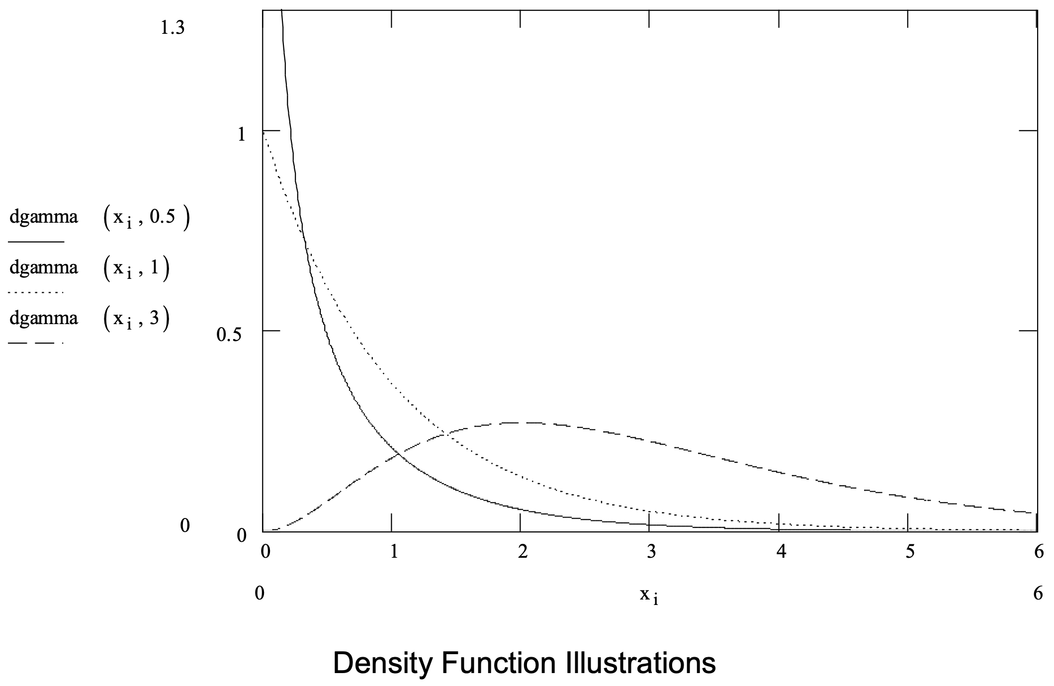
The Weibull and lognormal are possibilities as mentioned above. The gamma could be employed as well. A gamma distribution has two parameters: a shape parameter \(\ \alpha\) > 0 and a scale parameter \(\ \beta\) > 0. It is one of the most general and flexible ways to model a time delay. Note that the exponential distribution is a special case of the gamma distribution for \(\ \alpha\) = 1.

Figure 3-6: Summary of the Weibull Distribution.

Parameters:	Shape parameter, \(\ \alpha\) > 0, and a scale parameter, \(\ \beta\) > 0.
Range:	[0, \(\ \infty))
Mean:	\(\ \frac{\beta}{\alpha} \Gamma\left(\frac{1}{\alpha}\right),\ where\ Gamma\ is\ the\ gamma\ function.\)
Variance:	\(\ \frac{\beta^{2}}{\alpha}\left\{2 \Gamma\left(\frac{2}{\alpha}\right)-\frac{1}{\alpha}\left[\Gamma\left(\frac{1}{\alpha}\right)\right]^{2}\right\}\)
Densityfunction:	\(\ f(x)=\alpha \beta^{-\alpha} x^{\alpha-1} e^{-(x / \beta)^{\alpha}} ; x \geq 0\)
Distributionfunction:	\(\ F(x)=1-e^{-(x / \beta)^{\alpha}} ; x \geq 0\)
Application:	The Weibull distribution is used to model the time between equipment failures as well as operation times.

Figure 3-7: Summary of the Lognormal Distribution.

Parameters:	mean (\(\ \mu\)) and standard deviation (\(\ \sigma\)) of the normal distribution that results from taking the natural logarithm of the lognormal distribution
Range:	[0, \(\ \infty\))
Mean:	\(\ e^{\mu+o^{2} / 2}\)
Variance:	\(\ e^{2 \mu+o^{2}}\left(e^{o^{2}}-1\right)\)
Densityfunction:	\(\ f(x)=\frac{1}{x \sqrt{2 \pi o^{2}}} e^{\frac{-(\ln (x)-\mu)^{2}}{2 \sigma^{2}}} ; x>0\)
Distribution function:	No closed form
Application:	The lognormal distribution is used to model the time between equipment failures as well as operation times. By the central limit theorems, the lognormal distribution can be used to model quantities that are the products of a large number of other quantities.

The gamma distribution is summarized in Figure 3-8.

Figure 3-8: Summary of the Gamma Distribution

Parameters:	Shape parameter, \(\ \alpha\) > 0, and a scale parameter, \(\ \beta\) > 0.
Range:	[0, \(\ \infty\))
Mean:	\(\ \alpha * \beta\)
Variance:	\(\ \alpha * \beta^{2}\)
Density function:	\(\ f(x)=\frac{\beta^{-\alpha} x^{\alpha-1} e^{-(x / \beta)}}{\Gamma(\alpha)} ; x>0\)
Distribution function:	No closed form, except when \(\ \alpha\) is a positive integer.
Application:	The gamma distribution is the most flexible and general distribution for modeling operation times.

It is often argued that the simulation experiment should include the possibility of long operation, inspection, and transportation times. A single such time can have a noticeable effect on system operation since following entities wait for occupied resources. In this case, a Weibull, lognormal, or gamma distribution can be used since each extends to positive infinity.

A counter argument to the use of long delay times is that they represent special cause variation. Often special cause variation is not considered during the initial phases of system design and thus would not be included in the simulation experiment. The design phase often considers only the nominal dynamics of the system.

Controls are often used during system operation to adjust to long delay times. For example, a part requiring a long processing time may be out of specification and discarded after a pre- specified amount of processing is performed. Such controls can be included in simulation models if desired.

The normal distribution, by virtue of central limit theorems (Law, 2007), is useful in representing quantities that are the sum of a large number (25 to 30 at least) of other quantities. For example, a sales region consists of 100 convenience stores. Demand for a particular product in that region is the sum of the demands at each store. The regional demand is modeled as normally distributed. This idea is illustrated in the application study on automated inventory management.

A single operation can be used to model multiple tasks. In this case, the operation time represents the sum of the times to perform each task. If enough tasks are involved, the operation time can be modeled using the normal distribution.

The parameters of a normal distribution function are the mean (\(\ \mu\)) and the standard deviation (\(\ \sigma\)). Figure 3-8 shows several normal distribution density functions and summarizes the normal distribution.

Some quantities have to do with the number of something, such as the number of parts in a batch, the number of items a customer demands from inventory or the number of customers arriving between noon and 1:00 P.M. Such quantities can be modeled using the Poisson distribution.

Unlike the distributions previously discussed, the range of the Poisson distribution is only non- negative integer values. Thus, the Poisson is a discrete distribution. The Poisson has only one parameter, the mean.

Note that if the Poisson distribution is used to model the number of events in a time interval, such as the number of customers arriving between noon and 1:00 P.M., that the time between the events, arrivals, is exponentially distributed. In addition, the normal distribution can be used as an approximation to the Poisson distribution. The Poisson distribution is summarized in Figure 3- 9.

Some quantities can take one of a small number of values, each with a given probability. For example, a part is of type “1” with 70% probability and of type “2” with 30% probability. In these cases, the probability mass function is simply enumerated, e.g. p₁ = 0.70 and p₂ = 0.30. The enumerated probability mass function is summarized in Figure 3-10.

Figure 3-8: Summary of the Normal Distribution.

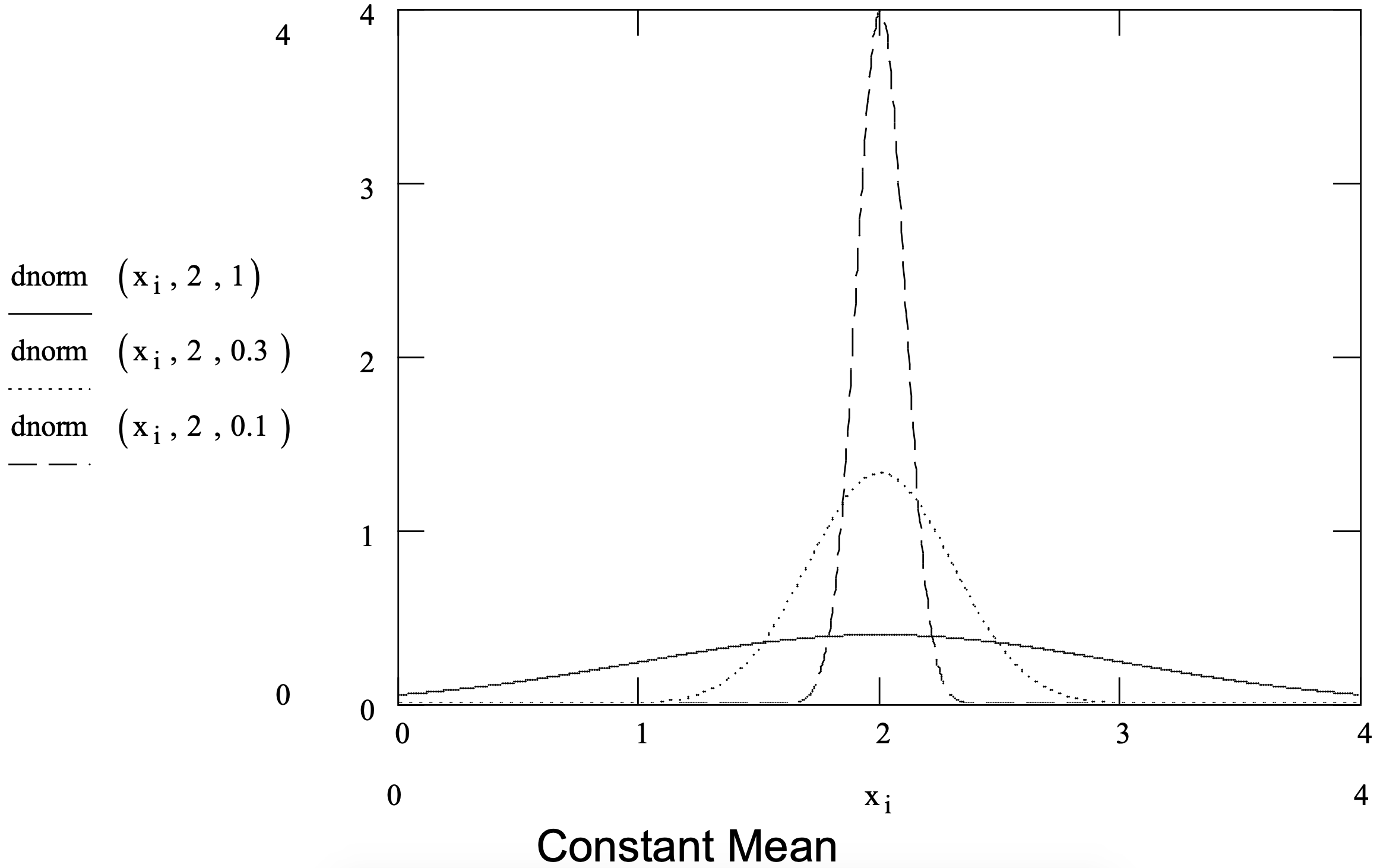
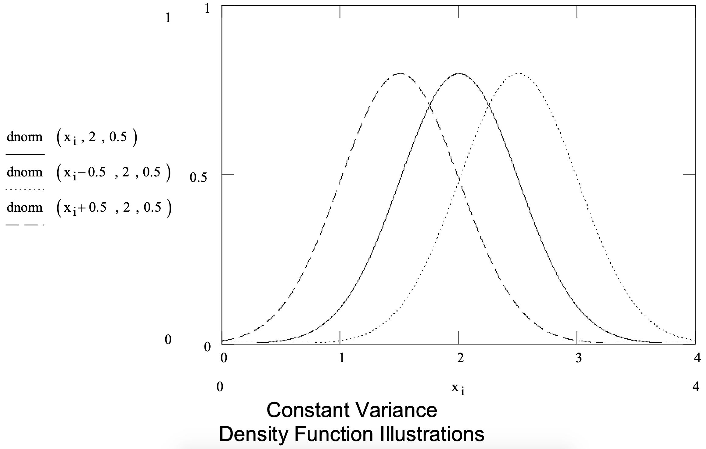
Parameters:	mean ( \(\ \mu\) ) and standard deviation ( \(\ \sigma\) )
Range:	(-\(\ \infty\), \(\ \infty\))
Mean:	\(\ \mu\)
Variance:	\(\ \sigma^{2}\)
Densityfunction:	\(\ f(x)=\frac{1}{\sqrt{2 \pi o^{2}}} e^{\frac{-(x-\mu)^{2}}{2 \sigma^{2}}}\)
Distribution function:	No closed form
Application:	By the central limit theorems, the normal distribution can be used to model quantities that are the sum of a large number of other quantities.

Figure 3-9: Summary of the Poisson Distribution

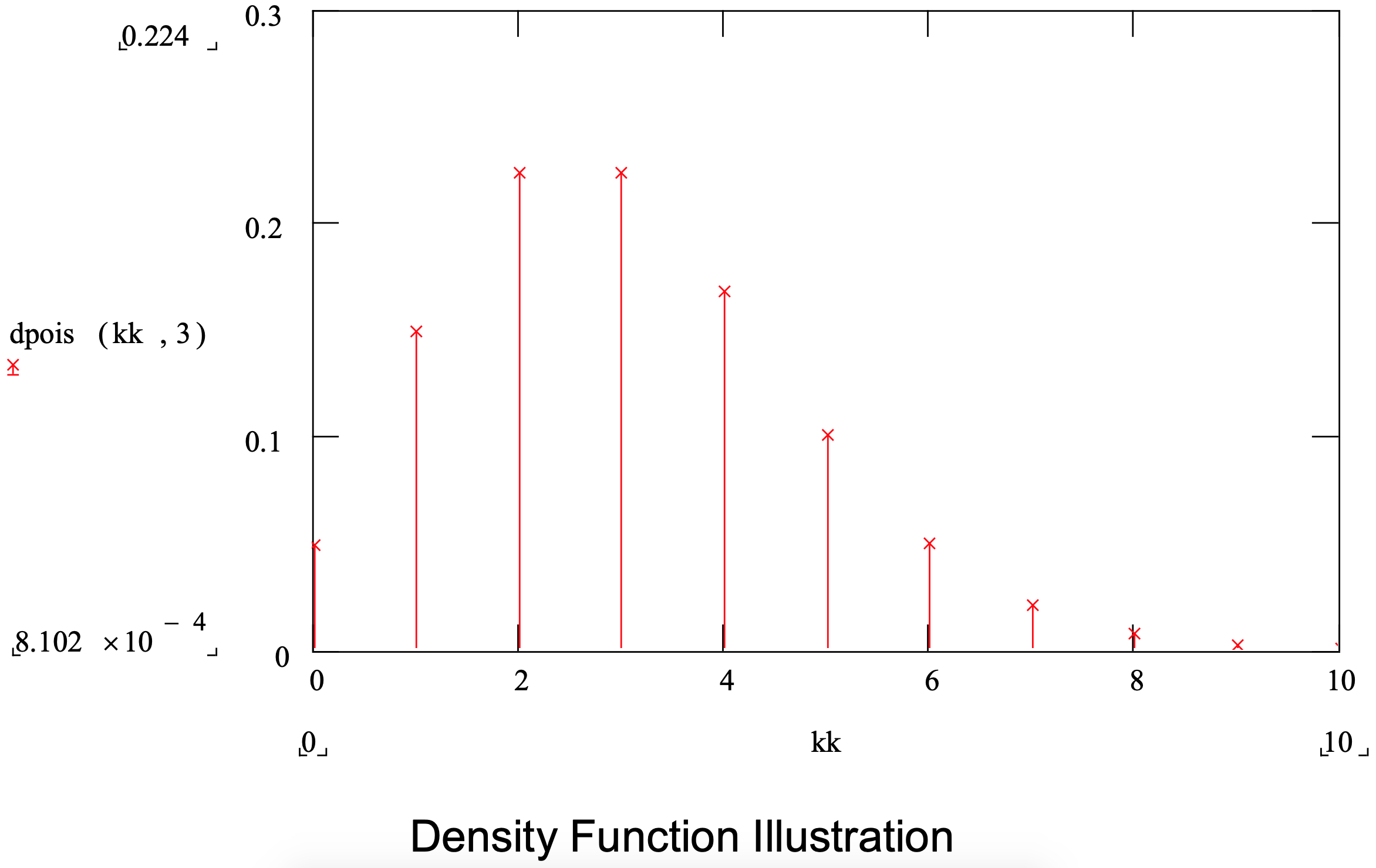
Parameter:	mean
Range:	Non-negative integers
Mean:	given parameter
Variance:	mean
Massfunction:	\(\ p(x)=\frac{e^{-\text {mean}} * \text {mean}^{x}}{\mathrm{x} !} ; x \text { is a non - negative integer }\)
Distributionfunction:	\(\ F(x)=e^{-m e a n} * \sum_{i=0}^{x} \frac{m e a n^{i}}{i !} ; x \text { is a non - negative integer }\)
Application:	The Poisson distribution is used to model quantities that represent the number of things such as the number of items in a batch, the number of items demanded by a single customer, or the number of arrivals in a certain time period.

Figure 3-10: Summary of the Enumerated Probability Mass Function

Parameter:	set of value-probability pairs (x,, pi), number of pairs, n
Range:	[minimum xi , maximum xi]
Mean:	\(\ \sum_{i=1}^{n} p_{i} * x_{i}\)
Variance:	\(\ \sum_{i=1}^{n} p_{i} *\left(x_{i}-\text { mean }\right)^{2}\)
Mass function:	\(\ p\left(x_{i}\right)=p_{i}\)
Distribution function:	\(\ F\left(x_{i}\right)=\sum_{k=1}^{i} p_{k}\)
Application:	An enumerated probability mass function is used to model quantities that represent the number of things such as the number of items in a batch and the number of items demanded by a single customer where the probability of each number of items is known and the number of possible values is small.

Law and McComas (1996) estimate that “perhaps one third of all data sets are not well represented by a standard distribution.” In this case, two options exist:

1. Form an empirical distribution function from the data set.
2. Fit a generalized functional form to the data set that has the capability of representing an unlimited number of shapes.

The former can be accomplished by using the frequency histogram of a data set to model a random quantity. The disadvantages of this approach are that the simulation considers only values within the range of the data set and in proportion to the cells that comprise the histogram.

One way to accomplish the latter is by fitting a Bezier function to the data set using an interactive Windows-based computer program as described by Flannigan Wagner and Wilson (1995, 1996).

3.3.3 A Software Based Approach to Fitting a Data Set to a Distribution Function

This section discusses the use of computer software in fitting a distribution function to data. Software should always be used for this purpose and several software packages support this task. The following three activities need to be performed.

1. Selecting the distribution family or families of interest.
2. Estimating the parameters of particular distributions.
3. Determining how well each distribution fits the data.

The distribution functions discussed in the preceding sections, beta or normal for example, are called families. An individual distribution is specified by estimating values for its parameters. There are two possibilities for selecting one or more distribution function families as candidates for modeling a random quantity.

1. Make the selection based on the correspondence between the situation being modeled and the theoretical properties of the distribution family as presented in the previous sections.

   For example, a large client buys a particular product from a supplier. The client supplies numerous stores from each purchase. The time between purchases is a random variable. Based on the theoretical properties of the distributions previously discussed, the time between orders could be modeled as using an exponential distribution and the number of units of product purchased could be modeled using a normal distribution.

2. Make the selection based on the correspondence between summary statistics and plots, such as a histogram, and particular density functions. Software packages such as ExpertFit [Law and McComas 1996, 2001] automatically compute and compare, using a relative measure of fit, candidate probability distributions and their parameters. In ExpertFit, the relative measure of fit is based on a proprietary algorithm that includes statistical methods and heuristics.

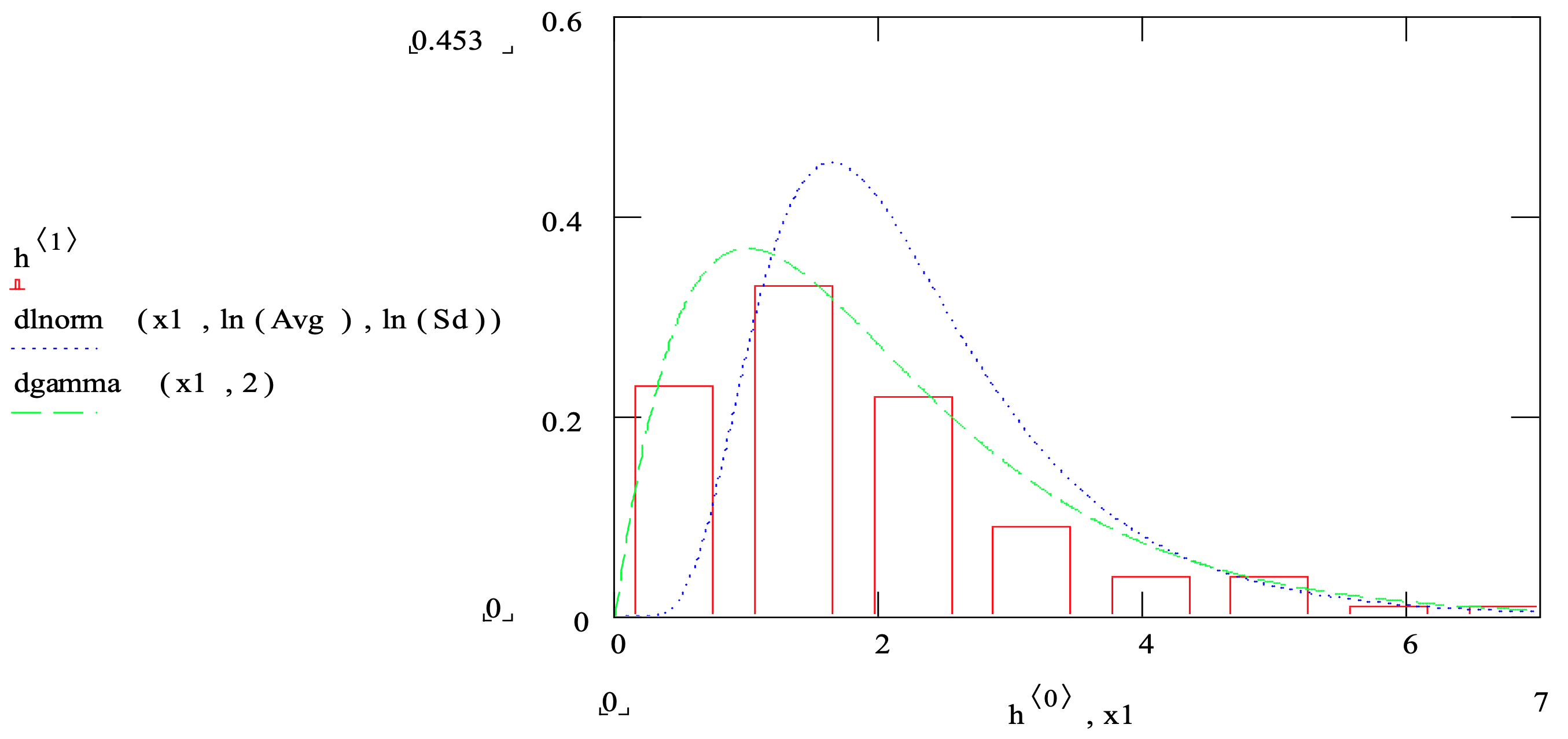
   For example, 100 observations of an operation time are collected. A histogram is constructed of this data. The mean and standard deviation are computed. Figure 3-11 shows the histogram on the same graph as a lognormal distribution and a gamma distribution whose mean and standard deviation were estimated from the data set. Note that the gamma distribution (dashed line) seems to fit the data much better than the lognormal distribution (dotted line).

Figure 3-11: Comparison of a Histogram with Gamma and Lognormal Density Functions

For some distributions, the estimation of parameters values is straightforward. For example, the parameters of the normal distribution are the mean and standard deviation that are estimated by the sample mean and sample standard deviation computed from the available data. For other distributions, the estimation of parameters is complex and may require advanced statistical methods. For example, see the discussion of the estimation procedure for the gamma distribution parameters in Law (2007). Fortunately, these methods are implemented in distribution function fitting software.

The third activity is to assess how well each candidate distribution represents the data and then choose the distribution that provides the best fit. This is called determining the “goodness-of-fit”. The modeler uses statistical tests assessing goodness of fit, relative and absolute heuristic measures of fit, and subjective judgment based on interactive graphical displays to select a distribution from among several candidates.

Heuristic procedures include the following:

1. Density/Histogram over plots – Plot the histogram of the data set and a candidate distribution function on the same graph as in Figure 3-11. Visually check the correspondence of the density function to the histogram.
2. Frequency comparisons – Compare the frequency histogram of the data with the probability computed from the candidate distribution of being in each cell of the histogram.

   For example, Figure 3-12 shows a frequency comparison plot that displays the sample data set whose histogram is shown in Figure 3-11 as well as the lognormal distribution whose mean and standard deviation were estimated from the data set. Differences between the lognormal distribution (solid bars) and the data set (non-solid bars) are easily seen.

   Figure 3-12: Frequency Comparison of a Data Set with a Lognormal Distribution

   

3. Distribution function difference plots – Plot the difference of the cumulative candidate distribution and the fraction of data values that are less than x for each x-axis value in the plot. The closer the plot tracks the 0 line on the vertical axis the better.

   For example, Figure 3-13 shows a distribution function difference plot comparing the sample data set whose histogram is displayed in Figure 3-11 to both the gamma and lognormal distributions whose mean and standard deviations were estimated from the data. The gamma distribution (solid line) appears to fit the data set much more closely that the lognormal distribution (dotted line).

   Figure 3-13: Distribution Function Difference Plot Comparison of a Data Set with a Gamma and a Lognormal Distribution

   

4. Probability plots – Use one of the many types of probability plots to compare the data set and the candidate distribution. One such type is as follows. Suppose there are n values in the data set. The following points, n in number, are plotted: ( i / n th percent point of the candidate distribution, the i th smallest value in the data set). These points when plotted should follow a 45 degree line. Any substantial deviation from this line indicates that the candidate distribution may not fit the data set.

   For example, Figure 3-14 shows a probability plot that compares the sample data set whose histogram is displayed in Figure 3-11 to both the gamma and lognormal distributions shown in the same figure. Note that the gamma distribution (solid line) tracks the 45 degree line better than does the lognormal distribution (dotted line) and both deviate from the line more toward the right tail.

   Figure 3-14: Probability Plot Comparison of a Data Set with Gamma and Lognormal Distributions

   

Statistical tests formally assess whether the data set that consists of independent samples is consistent with a candidate distribution. These tests provide a systematic approach for detecting relatively large differences between a data set and a candidate distribution. If no such differences are found, the best that can be said is that there is no evidence that the candidate distribution does not fit the data set.

The behavior of these tests depends on the number of values in the data set. For large values of n, the tests seem to always detect a significant difference between a candidate distribution and a data set. For smaller values of n, the tests detect only gross differences. This should be kept in mind when interpreting the results of the test.

The following tests are common and are typically performed by distribution function fitting software.

1. Chi-square test – formally compares a histogram of the data set with a candidate distribution as was done visually using a frequency comparison plot.
2. Kolmogorov-Smironv (K-S) test – formally compares an empirical distribution function constructed from the data set with a candidate cumulative distribution, which is analogous to the distribution function difference plot.
3. Anderson-Darling test – formally compares an empirical distribution function constructed from the data set with a candidate cumulative distribution function but is better at detecting differences in the tails of the distribution than the K-S test.

This chapter discusses how to determine the distribution function to use in modeling a random quantity. How this choice can affect the results of a simulation study has been illustrated. Some issues with obtaining and using data have been discussed. Selecting a distribution both using a data set and in the absence of data has been presented.

Problems

1. List the distributions that have a lower bound.
2. List the distributions that have an upper bound.
3. List the distributions that are continuous.
4. List the distributions that are discrete.
5. Suppose X is a random variable that follows a beta distribution with range [0,1]. A random variable, Y, is needed that follows a beta distribution with range [10, 100]. Give an equation for Y as a function of X.
6. Suppose data are not available when a simulation project starts.
   1. What three parameters are commonly estimated without data?
   2. An operation time is specified giving only two parameters: minimum and maximum. However, it is to be modeled using a triangular distribution. What would you do?
7. Consider the following data set: 1, 2, 2, 3, 4, 5, 7, 8, 9, 10, 11, 13, 15, 16, 17, 17, 18, 18, 18, 20, 20, 21, 21, 24, 27, 29, 30, 37, 40, 40. What distribution family appears to fit the data best? Use summary statistics and a histogram to assist you.
8. Hypothesize one or more families of distributions for each of the following cases:
   1. Time between customers arriving at a fast food restaurant during the evening dinner hour.
   2. The time till the next failure of a machine whose failure rate is constant.
   3. The time till the next failure of a machine whose failure rate increases in time.
   4. The time to manually load a truck based on the operational design of a system.

      You ask the system designers for the minimum, average, and maximum times.

   5. The time to perform a task with long task times possible.
   6. The distribution of job types in a shop.
   7. The number of items each customer demands.
9. What distribution function family appears to fit the following data set best? Use summary statistics and a histogram to assist you. Test your selection using the plots discussed in section 3.3.2.

   8.39	3.49	3.17	15.34	4.68	4.38	0.02	1.21
   3.56	0.50	4.38	2.53	20.61	2.78	2.66	32.88
   22.49	5.10	4.58	3.07	22.64	34.86	9.59	0.67
   12.24	3.25	34.07	5.43	14.72	5.84	15.37	21.20
   0.21	3.20	25.12	3.18	3.60	11.45	1.07	8.69
   0.46	9.16	10.71	3.75	1.54	0.65	3.68	10.46
   20.11	5.81	4.63	3.13	8.99	2.82	0.87	13.45
   10.10	12.57	22.67	3.55	5.68	29.07	0.62	25.23
   17.97	35.76	17.05	4.61	12.36	14.02	24.33	11.05
   1.10	4.56	9.51	7.31	23.33	5.81	3.48	3.23

10. What distribution function family appears to fit the following data set best? Use summary statistics and a histogram to assist you. Test your selection using the plots discussed in section 3.3.2.

    2373	2361	2390	2377	2333
    2327	2380	2373	2360	2382

11. Use the distribution function fitting software to solve problems 7, 9, and 10.