4.5: Design Elements Specific to Terminating Simulation Experiments

A terminating simulation experiment ends at a specified simulation time or event that is derived from the characteristics of the system under study and is stated as a part of the experiment design. This is the distinguishing characteristic of such as an experiment.

This section presents the design elements that are specific to terminating simulation experiments. These include setting initial conditions, specifying the number of replications of the experiment, and specifying the ending time or event of the simulation.

4.5.1 Initial Conditions

To begin a simulation, the initial values of the state variables and the initial location in the model of any entities, along with their attribute values, must be specified. Together, these are called the initial conditions.

In a terminating simulation, the initial conditions should be the same as conditions that occur in the actual system (Law, 2007). The work of Wilson and Pritsker (1978) leads toward using the modal or, at least, frequently occurring conditions. This must be done to ensure there is not a statistically significant greater portion of performance measure values in any given range gathered from the simulation than would occur in the actual system. Thus, statistical bias is collecting performance measure values that could not have occurred, or in greater (lesser) proportion in one range than could have occurred, in the actual system.

Consider again the two work stations in a series model. For example, suppose it is known that parts are almost always in the buffer of workstation A and of workstation B. Thus possible initial conditions are:

1. The workstation A resource is in the BUSY state processing one part.
2. The workstation B resource is in the BUSY state processing one part.
3. Two parts are in the buffer of workstation A.
4. Two parts are in the buffer of workstation B.

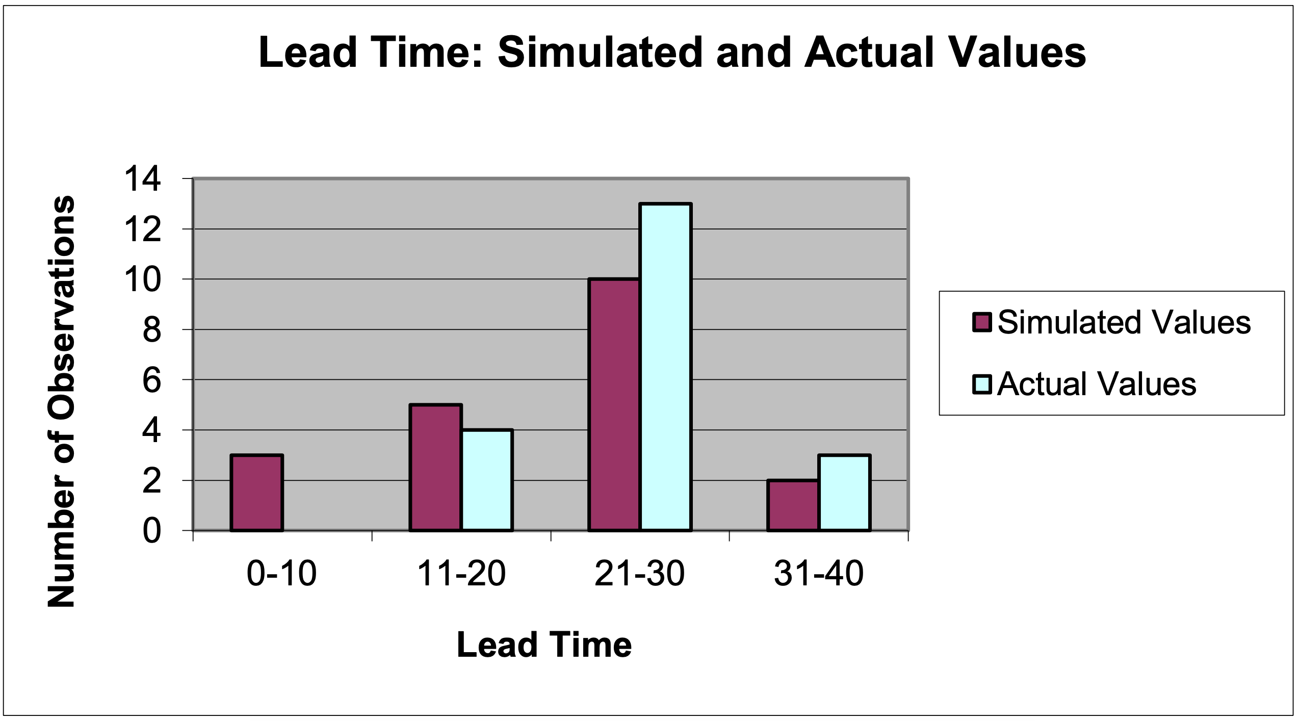
Note that the time spent at either workstation by a part will consist of the time spent in the input buffer plus the operation time. If the simulation experiment begins with no parts in either input buffer, the time the first part spends at each workstation is equal to the operation time because the time spent in the input buffer will be zero. The observed lead time for this part will be less than for any part processed by the actual system.

Statistical bias is illustrated in Figure 4-2 that shows example histograms of part time in the system collected from the actual system and from a simulation. The simulation has improper initial conditions of no parts at the workstation. Some of the simulation observations are biased low. Calculations of statistics based on statistically biased observations may also be biased and inaccurate conclusions about problem root causes or the performance of proposed solutions drawn.

The initial conditions must be specified as a part of the experimental design and must be actual conditions that occur in the system.

Figure 4-2: Illustration of Statistical Bias

4.5.2 Replicates

This section discusses the idea of replication to construct independent observations of simulation performance measures. Replicates of a simulation experiment differ from each other only in the sample values of the quantities modeled by probability distributions. Replicates are treated as independent of each other since the sample values exhibit no statistical correlation.

Each replicate is one possibility of how the random behavior of the system actually occurred. Multiple possibilities for system behavior should be examined in detail to draw conclusions about the effectiveness of system scenarios in meeting solution objectives.

Consider again the two work stations in a series model. There is a stream of sample values for the time between arrivals and another stream for operation times at workstation A. A replicate is defined by the particular samples taken in these two streams. Examining system performance for other streams of the time between arrivals and of service times is necessary. These other streams define additional replicates.

Observations of the same performance measure from different replicates are statistically independent of each other. In addition, performance measure observations from different replicates are identically distributed for the same reason. Thus replication is one way of constructing independent observations for statistical analysis. However, since performance measures may be arbitrarily defined, the underlying probability distribution of the performance measure observations cannot be determined in general.

During each replicate, one or more observations of the values of a performance measure are made. For example, the number of entities that complete processing in the two work stations in series model is incremented each time processing is finished, the lead time is recorded each time an entity completes processing, and the number of entities in either workstation buffer is updated each time an entity arrives at a workstation as well as each time an entity begins processing.

For the reasons discussed in section 4.3, each replicate can produce only one independent sample, xi. This independent sample is often a statistic computed from the observations of a performance measure, usually the average, minimum, or maximum. For example, one average of the number in the buffer at a workstation A is computed from all of observations made during one replicate. This average is one independent sample of the average number in the buffer.

Statistical summaries are estimated from the x’s. These summaries typically include the i

average, standard deviation, minimum, and maximum. Confidence intervals are also of interest.

In summary, each simulation experiment consists of n replicates. Within each replicate and for each performance measure, one or more observations are made. From the observations, one or more statistics are typically computed. Each such statistic is the independent observation, xi, produced by the replicate.

For example, a simulation experiment concerning the two work stations in a series model could consist of 20 replicates. The number of entities in the workstation A buffer could be observed. Each time the number in the buffer changes an observation is made. The average number in the buffer as well as the maximum number in the buffer is computed. There are 20 independent observations of the average number in the buffer as well as 20 independent observations of the maximum number in the buffer.

The number of replicates initially made is generally determined by experience and the total amount of real (“clock”) time needed to compute the simulation. Most of the time, this number is in the range 10-30. More replicates may be needed if the width of a confidence interval computed from the performance measure observations is considered to be too wide. Confidence interval estimation is discussed later in this chapter.

The number of replications of the simulation experiment must be specified.

4.5.3 Ending the Simulation

This section discusses the time or condition that determines when to end a replicate.

An ending time for a replicate arises naturally from an examination of most systems. A manufacturer wants to know if its logistic equipment will suffice for the next budget period of one year. So the end of the budget year becomes the simulation ending time. A fast food restaurant does most of its business from 11:30 A.M to 12:30 P.M. Thus the simulation ending time is one hour. The experiment for a production facility model could cover the next planning period of three months. After that time, new levels of demand may occur and perhaps new production strategies implemented. The simulation experiment for a production facility could end when 100 parts are produced.

4.5.4 Design Summary

The specification of design elements for a terminating simulation experiment can be accomplished by completing the template shown in Table 4-1.

Table 4-1: Terminating Simulation Experiment Design
Element of the Experiment	Values for a Particular Experiment
Model Parameters and Their Values
Performance Measures
Random Number Streams
Initial Conditions
Number of Replicates
Simulation End Time / Event

Consider a terminating simulation experiment for the two workstations in a series model. The time between arrivals and the operation time at workstation A are modeled using probability distributions. Performance measures include the number in the buffer at each workstation, the state of the each workstation (BUSY or IDLE), and entity lead time. The model parameter is the machine used at workstation A, either the current machine with operation time uniformly distributed between 5 and 13 seconds or a new machine with operation time uniformly distributed between 7 and 11 seconds. The initial conditions are two items in each buffer and both workstations busy. Twenty replicates will be made for the planning horizon of one work week. The experimental design is shown in Table 4-2.

Table 4-2: Simulation Experiment Design for the Two Workstations in Series Model
Element of the Experiment	Values for a Particular Experiment
Model Parameters and Their Values	Workstation A Machine: Current vs. New
Performance Measures	Number in the buffer at each workstation State of each workstation Lead Time
Random Number Streams	Time between arrivals Operation Time
Initial Conditions	Two entities in each buffer One entity in service at each workstation (State of each workstation resource is BUSY)
Number of Replicates	20
Simulation End Time / Event	1 week (40 hours)