4.6: Examining the Results for a Single Scenario

This section presents a strategy for examining the simulation results of a single system scenario as defined by one set of model parameter values. Results are examined to gain an understanding of system behavior. Statistical evidence in the form of confidence intervals is used to confirm that what is observed is not just due to the random nature of the simulation model and experiment and thus provides a valid basis for understanding system behavior.

Simulation results are displayed and examined using graphs and histograms as well as summary statistics such as the mean, standard deviation, minimum, and maximum. Patterns of system behavior are identified if possible. Animation is used to display the time dynamics of the simulation. This is in accordance with principle 8: Looking at all the simulated values of performance measures helps.

How the examination of simulation results is successfully accomplished is an art as stated in principle 1. Thus, this topic will be further discussed and illustrated in the context of each application study.

The discussion in this session is presented in the context of the two work stations in a series model.

4.6.1 Graphs, Histograms, and Summary Statistics

Observed values for each performance measure can be examined via plots, histograms, and summary statistics. To illustrate, each of these will be shown for the number of entities in the buffer of workstation A in the two workstations in a series model.

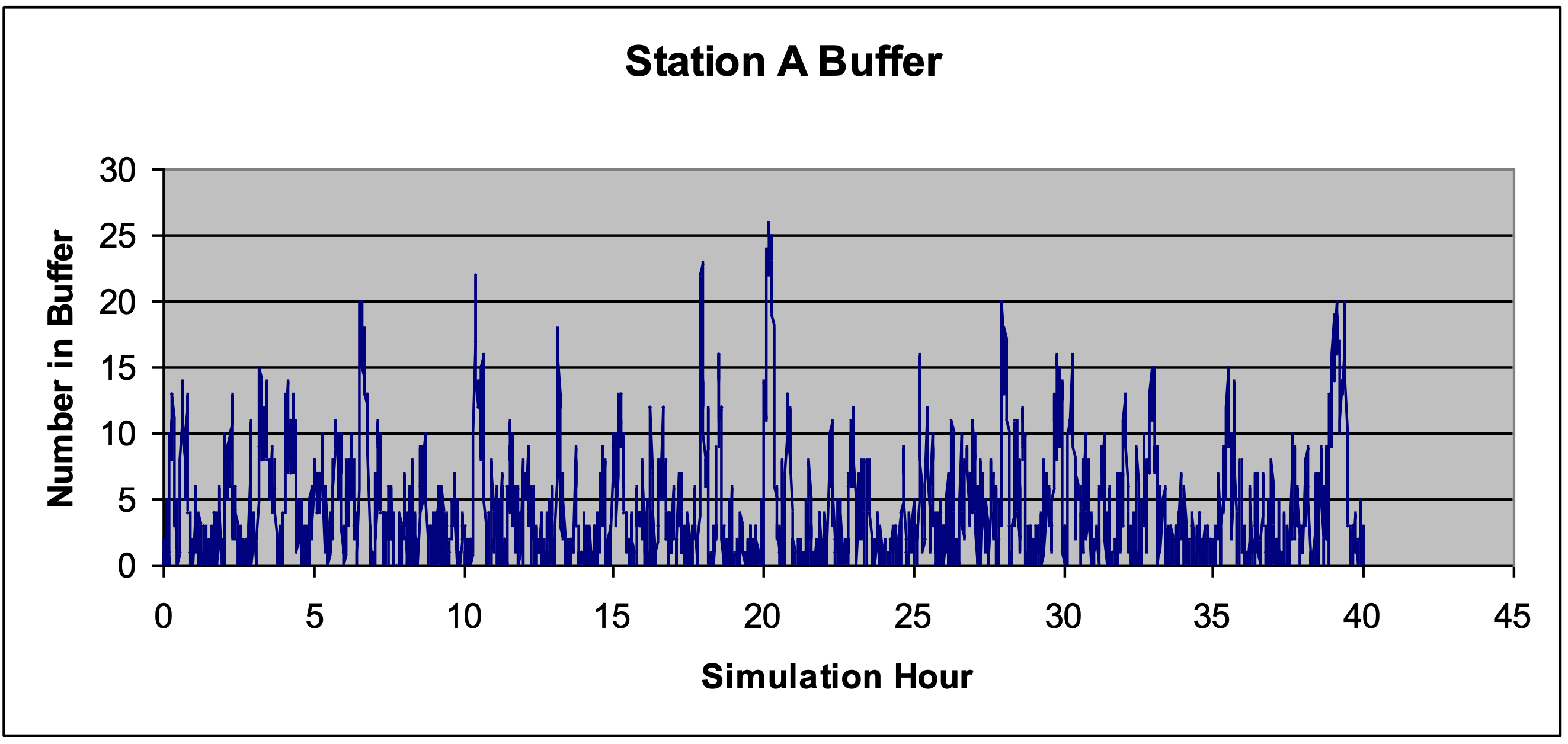
A plot of the observed values of the number in this buffer from replicate one of the simulation experiment defined in Table 4-2 is shown in Figure 4-3. The x-axis is simulated time and the y- axis is the number in the buffer of workstation A. Note from the plot that most of the time the number in the buffer varies between 0 and 10. However, there are several occasions that the number in the buffer exceeds 20. This shows high variability at workstation A.

Figure 4-3: Plot of the Number of Entities in the Workstation A Buffer

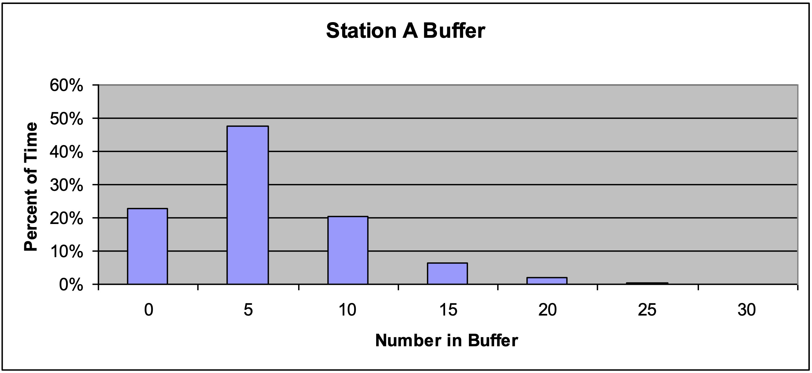
A histogram of the same observations is shown in Figure 4-4. The percent of time that a certain number of entities is in the buffer is shown on the y-axis. The number of entities is shown on the x-axis. Note that about 91% of the time there are 10 or less entities in the buffer of workstation A. However about 9% of the time there are more than 10 entities in the buffer.

It would be wise to examine these same graphs from other replicates to see if the same pattern of behavior is observed. If the software capability is available, a histogram combining the observations from all of the replicates would be of value.

Figure 4-4: Histogram of the Number of Entities in the Workstation A Buffer

Summary statistics can be computed from the observations collected in each replicate. However, these observations are likely not independent, so their standard deviation is not very useful. The average, minimum, and maximum of the observations of the number in the buffer of workstation A from replicate 1 are given in Table 4-3. The average number of entities is relatively low but the maximum again shows the high variability in the number in the buffer.

Table 4-3: Summary Statistics for the Number of Entities in the Buffer of Workstation A – Replicate 1
Statistic	Value
Average	4.1
Minimum	0
Maximum	26

As was previously discussed, one independent observation each of the average, minimum, and maximum is generated by each replicate. Suppose the average and maximum number in the buffer of workstation A are of interest. The average corresponds to the average work-in-process (WIP) at the workstation and the maximum to the buffer capacity needed at the workstation. Table 4-4 summarizes the results for 20 replicates. The average ranges from 3.1 to 6.6 with an overall average of 4.4. This shows that the average number in the buffer has little variability. The maximum shows significant variability ranging from 21 to 43 with an average of 31.

Table 4-4: Summary Statistics for the Number of Entities in the Buffer of Workstation A – Replicate 1 through 20
Replicate	Average Number in the Workstation A Buffer	Maximum Number in the Workstation A Buffer
1	4.1	28
2	4.6	27
3	4.1	30
4	3.2	24
5	3.8	24
6	4.3	29
7	4.0	25
8	4.4	34
9	4.3	40
10	4.1	28
11	4.1	26
12	4.5	38
13	4.5	31
14	4.3	30
15	4.8	37
16	4.2	28
17	5.2	40
18	4.3	38
19	4.3	26
20	4.4	36
Average	4.3	31.0
Std. Dev.	0.39	5.4
Minimum	3.2	24
Maximum	5.2	40

4.6.2 Confidence Intervals

One purpose of a simulation experiment is to estimate the value of ta parameter or characteristic of the system of interest such as the average or maximum number in the buffer of workstation A. The actual value of such a parameter or characteristic is most likely unknown. Both a point estimator and an interval estimator are needed. The point estimator should be the center point of the interval.

The average of the set of independent and identically distributed observations, one from each replicate, serves as a point estimator. For example, the values in the “average” row of Table 4-4 are point estimators, the first of the average WIP in the buffer of workstation A and the second of the needed buffer capacity.

The confidence interval estimation procedures recommend by Law (2007) will be used to provide an interval estimator. The t-confidence interval given by equation 4-1 is recommended.

\begin{align}P\left(\bar{X}-t_{1-\alpha / 2, n-1} * \frac{s}{\sqrt{n}} \leq \mu \leq \bar{X}+t_{1-\alpha / 2, n-1} * \frac{s}{\sqrt{n}}\right) \approx 1-\alpha\tag{4-1}\end{align}

where \(\ t_{1-\alpha / 2, n-1}\) is the \(\ 1-\alpha / 2\) percentage point of the Student’s t distribution with n-1 degrees of freedom, n is the number of replicates, \(\ \bar{X}\) is the average (the values on the “average” row of Table 4-4 for example), and s is the standard deviation (the values on the “std. dev.” row of Table 4-4 for example). The \(\ \approx\) sign means approximately. The symbol \(\ \mu\) represents the actual but unknown value of the system parameter or characteristic of interest.

The result of the computations using equation 4-1 is the interval shown in equation 4-2:

\begin{align}\text{(lower bound} \leq \mu \leq \text{upper bound) with}\ 1 - \alpha\ \text{confidence}\tag{4-2}\end{align}

where

\begin{align}\text { lower bound }=\bar{X}-t_{1-\alpha / 2, n-1} * \frac{s}{\sqrt{n}}\tag{4-3}\end{align}

\begin{align}\text { upper bound }=\bar{X}+t_{1-\alpha / 2, n-1} * \frac{s}{\sqrt{n}}\tag{4-4}\end{align}

Equations 4-1 and 4-2 show the need to distinguish between probability and confidence. Understanding this difference may require some reflection since in everyday, non-technical language the two ideas are often used interchangeably and both are expressed as a percentage.

A probability statement concerns a random variable. Equation 4-1 contains the random variables \(\ \bar{X}\) and s and thus is a valid probability statement. The interpretation of equation 4-1 relies on the long run frequency interpretation of probability and is as follows: If a very large number of confidence intervals are constructed using equation 4-1, the percentage of them that include the actual but unknown value of \(\ \mu\) is approximately \(\ 1-\alpha\). This percentage is called the coverage.

The interval expressed in equation 4-2 contains two numeric values: lower bound and upper bound plus the constant \(\ \mu\) whose value is unknown. Since there are no random variables in equation 4-2, it cannot be a probability statement. Instead, equation 4-2 is interpreted as a statement of the degree of confidence \(\ (1-\alpha)\) that the interval contains the value of the system parameter or characteristic of interest. Typical values for \(\ (1-\alpha)\) are 90%, 95%, and 99%. A higher level of confidence implies more evidence that the interval contains the value of \(\ \mu\).

Some thoughts on how to interpret the level of confidence with respect to the kind of evidence provided is worthwhile. Keller (2001) suggests the following, which will be used in this text.

Table 4-5. Interpretation of Confidence Values
Confidence \(\ (1-\alpha)\) Range	Interpretation
\(\ (1-\alpha) \geq\) 99%	Overwhelming evidence
95% \(\ \geq(1-\alpha)>\) 99%	Strong evidence
90% \(\ \geq(1-\alpha)>\) 95%	Weak evidence
90% \(\ >(1-\alpha)\)	No evidence

Note that the higher the level of confidence the greater the value of \(\ t_{1-\alpha / 2, n-1}\) and thus the wider the confidence interval. A narrow confidence interval is preferred so that the value of \(\ \mu\) is more precisely bounded. However, it is clear that a high level of confidence must be balanced with the desire for a narrow confidence interval.

Why equation 4-1 is approximate and not exact is worthy of discussion. For equation 4-1 to be exact, the observations on which the confidence interval computations are based must come from a normal distribution as well as being independent and identically distributed. As was previously discussed, the latter two conditions are met by the definition of a replicate while the first condition cannot be guaranteed since the performance measures in a simulation are arbitrarily defined.

Thus, equation 4-1 is approximate. Approximate means that the coverage produced using equation 4-1 will likely be less than \(\ 1-\alpha\).

Given that equation 4-2 provides only an approximate (not exact) level of confidence (not a probability), it is natural to ask why it should be used. Law (2007) concludes that experience has shown that many real-world simulations produce observations of the type for which equation 4-1 works well, that is the coverage produced using equation 4-1 is close enough to \(\ 1-\alpha\) to be useful in conducting simulation studies. In the same way, Vardeman and Jobe (2001) state that confidence intervals in general have great practical use, even though no probability statement can be made as to whether a particular interval contains the actual value of the system characteristic or parameter of interest. Since confidence intervals seem to work well in general and in simulation studies, they will be used throughout this text.

As an example, Table 4-6 contains the 99% confidence intervals computed from equation 4-2 for the average and maximum number of entities in the buffer of workstation A based on the results shown in Table 4-4.

Table 4-6: 99% Confidence Intervals for the Number of Entities in the Buffer of Workstation A Based on 20 Replicates
	Average Number in the Workstation A Buffer	Maximum Number in the Workstation A Buffer
Average	4.3	31.0
Std. Dev.	0.39	5.4
99% CI – Lower Bound	4.0	27.5
99% CI – Upper Bound	4.5	34.4

The confidence interval for the average is small. It would be safe to conclude that the average number in the buffer of workstation A was 4 (in whole numbers). The confidence interval for the maximum number in the buffer ranges from 27 to 34 (in whole numbers). If this range is deemed too wide to establish a buffer size additional replicates, say another 20, could be made.

4.6.3 Animating Model Dynamics

As discussed in chapter 1, simulation models and experiments capture the temporal dynamics of systems. However, reports of models and experimental behavior are often confined to static mediums such as reports and presentations like those shown in the preceding sections. The simulation process includes system experts and managers who may not be knowledgeable about modeling methods and may be skeptical that a computer model can represent the dynamics of a complex system. In addition, complex systems may include complex decision rules. All behavioral consequences resulting from these rules may be difficult to predict.

Addressing these concerns involves answering the question: What system behavior was captured in the model? One very effective way of meeting this requirement is seeing the behavior graphically. This is accomplished using animation.

Typical ways of showing simulated behavior using animation follow:

1. State of a resource with one unit: The resource is represented as a graphical object that physically resembles what the resource models. For example, if the resource models a lathe, then the object looks like a lathe. Each state of the resource corresponds to a different color. For example, yellow corresponds to IDLE, green to BUSY, and red to BROKEN. Color changes during the animation indicate changes in the state of the resource in the simulation.
2. Entities: An entity is represented in the frame as a graphical object that physically resembles what the entity models. Different colors may be used to differentiate entities with different characteristics. For example if there are two types of parts, graphical objects representing part type 1 may be blue and those representing part type 2 may be white.
3. Number of entities in a buffer: A graphical object, which may be visually transparent, represents the buffer. An entity graphical object is placed in the same location as the buffer graphical object whenever an entity joins the buffer in the simulation. The buffer graphical object accommodates multiple entity graphical objects.
4. Material transportation: Any movement, such as between workstations, of entities in the simulation can be shown on the animation. The location of an entity graphical object can be changed at a rate proportional to the speed or time duration of the movement. Movement of material handling equipment can be shown in a similar fashion. As for other resources, a piece of material handling equipment is represented by a graphical object that resembles that piece of equipment. For example, a forklift is represented by a graphical object that looks like a forklift.

An animation of the two-stations in a series system should be viewed at this time.