9.2: Traditional Inventory Models

9.2.1 Trading off Number of Setups (Orders) for Inventory

Consider the following situation, commonly called the economic order quantity problem. A product is produced (or purchased) to inventory periodically. Demand for the product is satisfied from inventory and is deterministic and constant in time. How many units of the product should be produced (or purchased) at a time to minimize the annual cost, assuming that all demand must be satisfied on time? This number of units is called the batch size.

The analysis might proceed upon the following lines.

1. What costs are relevant?
   1. The production (or purchase) cost of each unit of the product is sunk, that is the same no matter how many are made at once.
   2. There is a fixed cost per production run (or purchase) no matter how many are made.
   3. There is a cost of holding a unit of product in inventory until it is sold, expressed in $/year.

      Holding a unit in inventory is analogous to borrowing money. An expense is incurred to produce the product. This expense cannot be repaid until the product is sold. There is an "interest charge" on the expense until it is repaid. This is the same as the holding cost. Thus, the annual holding cost per unit is often calculated as the company minimum attractive rate of return times the cost of one unit of the product.

2. What assumptions are made?
   1. Production is instantaneous. This may or may not be a bad assumption. If product is removed from inventory once per day and the inventory can be replenished by a scheduled production run of length one day every week or two, this assumption is fine. If production runs cannot be precisely scheduled in time due to capacity constraints or competition for production resources with other products or production runs take multiple days, this assumption may make the results obtained from the model questionable.
   2. Upon completion of production, the product can be placed in inventory for immediate delivery to customers.
   3. Each production run incurs the same fixed setup cost, regardless of size or competing activities in the production facility.
   4. There is no competition among products for production resources. If the production facility has sufficient capacity this may be a reasonable assumption. If not, production may not occur exactly at the time needed.

The definitions of all symbols used in the economic order quantity (EOQ) model are given in Table 9-1.

Table 9-1: Definition of Symbols for the Economic Order Quantity Model
Term	Definition
Annual demand rate (D)	Units demanded per year
Unit production cost (c)	Production cost per unit
Fixed cost per batch (A)	Cost of setting up to produce or purchase one batch
Inventory cost per unit per year (h)	h = i * c where i is the corporate interest rate
Batch size (Q)	Optimal value computed using the inventory model
Orders per year (F)	D/Q
Time between orders	1/F = Q/D
Cost per year	Run (order) setup cost + inventory cost = A * F + h * Q/2

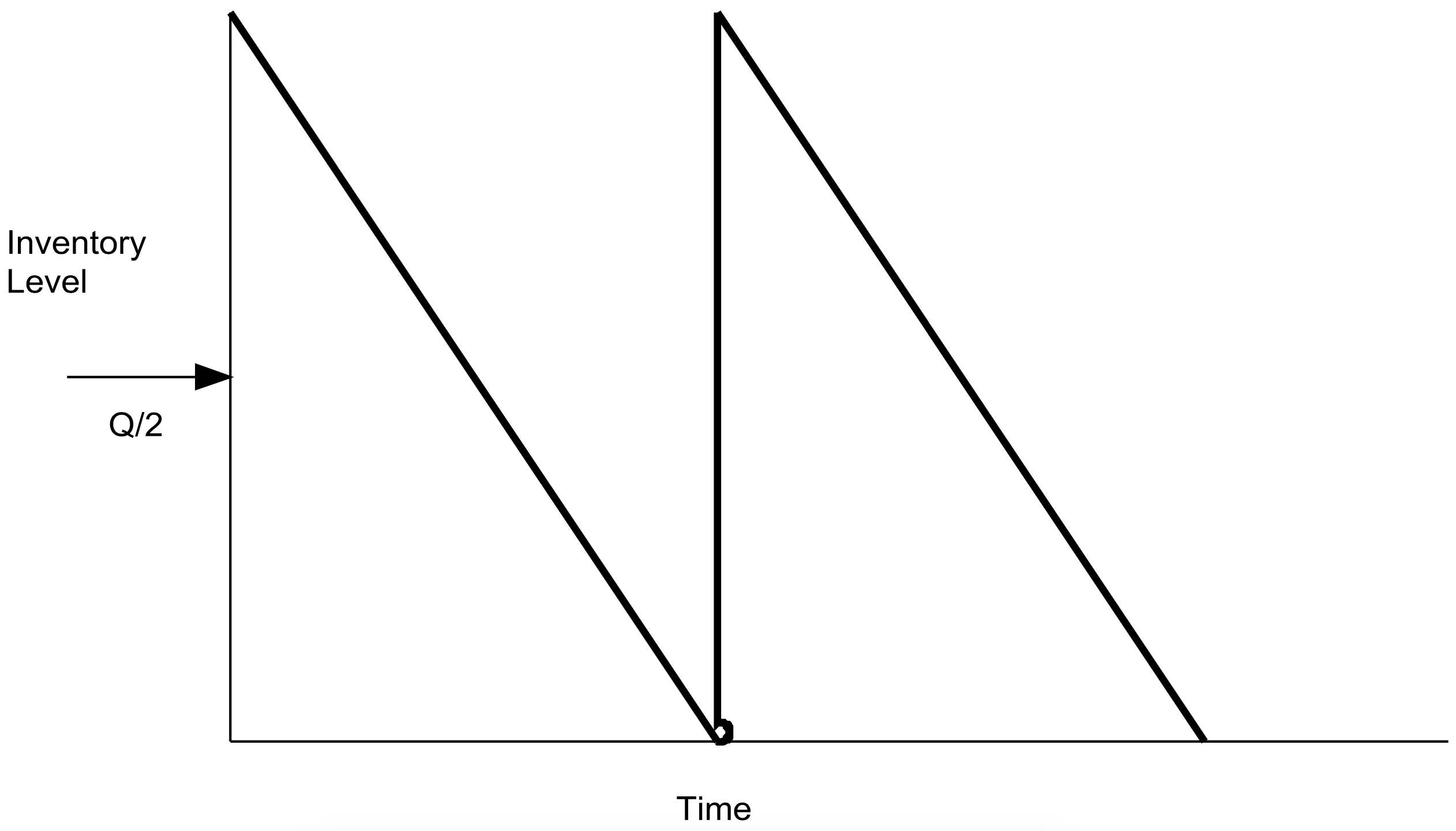
The cost components of the model are the annual inventory cost and the annual cost of setting up production runs. The annual inventory cost is the average number of units in inventory times the inventory cost per unit per year. Since demand is constant, inventory declines at a constant rate from its maximum level, the batch size Q, to 0. Thus, the average inventory level is simply Q/2. This idea is shown in Figure 9-1.

Figure 9-1: Inventory Level for EOQ Model

The number of production runs (orders) per year is the demand divided by the batch size. Thus the total cost per year is given by equation 9-1.

\begin{align}Y(Q)=h * \frac{Q}{2}+A * \frac{D}{Q}\tag{9-1}\end{align}

Finding the optimal value of Q is accomplished by taking the derivative with respect to Q, setting it equal to 0 and solving for Q. This yields equation 9-2.

\begin{align}Q^{*}=\sqrt{\frac{2 * A * D}{h}}=\sqrt{\frac{A}{h}} * \sqrt{2 * D}\tag{9-2}\end{align}

Notice that the optimal batch size Q depends on the square root of the ratio of the fixed cost per batch, A, to the inventory holding cost, h. Thus, the cost of a batch trades off with the inventory holding cost in determining the batch size.

Other quantities of interest are the number of orders per year (F) and the time between orders (T).

\begin{align}F^{*}=D / Q^{*}\tag{9-3}\end{align}

\begin{align}T^{*}=1 / F^{*}=Q^{*} / D\tag{9-4}\end{align}

It is important to note that:

Mathematical models help reveal tradeoffs between competing system components or parameters and help resolve them.

Even if values are not available for all model parameters, mathematical models are valuable because they give insight into the nature of tradeoffs. For example in equation 9- 2, as the holding cost increases the batch size decreases and more orders are made per year. This makes sense, since an increase in inventory cost per unit should lead to a smaller average inventory.

As the fixed cost per batch increases, batch size increases and fewer orders are made per year. This makes sense since an increase in the cost fixed cost per batch results in fewer batches.

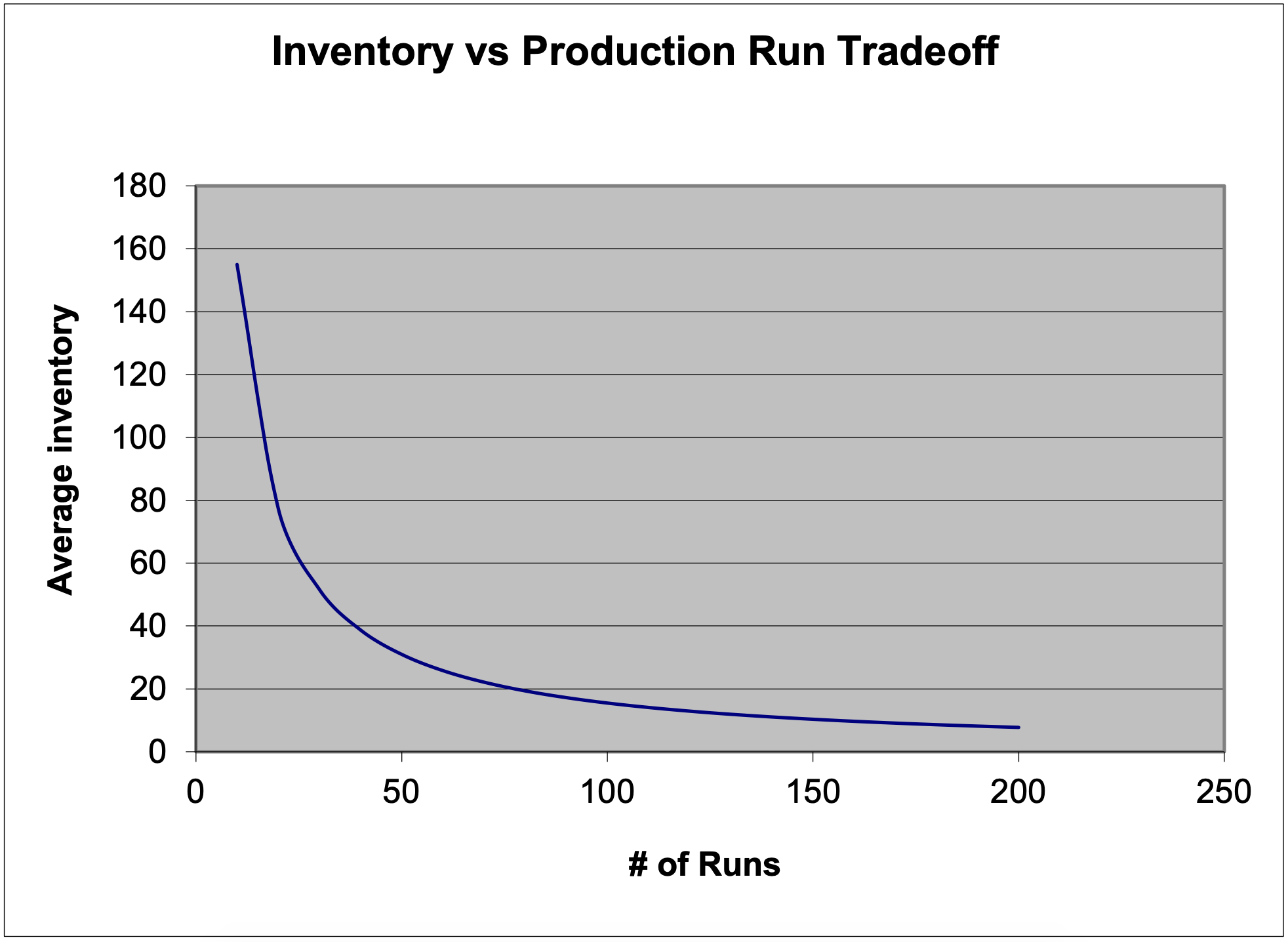
Suppose cost information is unknown and cannot be determined. What can be done in this application? One approach is to construct a graph of the average inventory level versus the number of production runs (orders) per year. An example graph is shown in Figure 9-2. The optimal tradeoff point is in the "elbow" of the curve. To the right of the elbow, increasing the number of production runs (orders) does little to lower the average inventory. To the left of the elbow, increasing the average inventory does little to reduce the number of production runs (orders).

In Figure 9-2, an average inventory of about 20 to 40 units leads to about 40 to 75 production runs a year. This suggests that optimal batch size can be changed within a reasonably wide range without changing the optimal cost very much. This can be very important as batch sizes may be for practical purposes restricted to a certain set of values, such as multiples of 12, as order placement could be restricted to weekly or monthly.

Example. Perform an inventory versus batch size analysis on the following situation. Demand for medical racks is 4000 racks per year. The production cost of a single rack is $250 with a production run setup cost of $500. The rate of return used by the company is 20%. Production runs can be made once per week, once every two weeks, or once every four weeks.

The optimal batch size (number of units per production run) is given by equation 9-2:

\(\ Q^{*}=\sqrt{\frac{2 * A * D}{h}}=\sqrt{\frac{2 * 500 * 4000}{250 * 20 \%}}=283\)

Figure 9- 2: Inventory versus Production Run Tradeoff Graph

The number of production runs per year and the time between production runs is given by equations 9-3 and 4:

\(\ F^{*}=D / Q^{*}=14.1\)

\(\ T^{*}=1 / F^{*}=Q^{*} / D=3.7 \text { weeks }\)

The optimal cost is given by equation 9-1:

\(\ Y\left(Q^{*}\right)=h * \frac{Q^{*}}{2}+A * \frac{D}{Q^{*}}=250 * 20 \% * \frac{283}{2}+500 * 14.1=7075+7071=14146\)

Applying the constraint on the time between production runs yields the following.

\(\ T^{\prime}=4\ weeks\)

\(\ F^{\prime}=52\ weeks\ /\ 4\ weeks =13\)

\(\ Q^{\prime}=4000 \ /\ F^{\prime}=308\)

\(\ Y\left(Q^{\prime}\right)=h * \frac{Q^{\prime}}{2}+A * \frac{D}{Q^{\prime}}=250 * 20 \% * \frac{308}{2}+500 * 13=7700+6500=14200\)

Note that when the optimal value of Q is used the inventory cost and the setup cost of production runs are approximately equal. When the constrained value is used, the inventory cost increases since batch sizes are larger but the setup cost decreases since fewer production runs are made. The total cost is about the same.

9.2.2 Trading Off Customer Service Level for Inventory

Ideally, no inventory would be necessary. Goods would be produced to customer order and delivered to the customer in a timely fashion. However, this is not always possible. Wendy's an cook your hamburger to order but a Christmas tree cannot be grown to the exact size required while the customer waits on the lot. In addition, how many items customers demand and when these demands will occur is not known in advance and is subject variation

Keeping inventory helps satisfy customer demand on-time in light of the conditions described in the preceding paragraph. The service level is defined as the percent of the customer demand that is met on time.

Consider the problem of deciding how many Christmas trees to purchase for a Christmas tree lot. Only one order can be placed. The trees may be delivered before the lot opens for business. How many Christmas trees should be ordered if demand is a normally distributed random variable with known mean and standard deviation?

There is a trade-off between:

1. Having unsold trees that are not even good for firewood.
2. Having no trees to sell to a customer who would have bought a tree at a profit for the lot.

Relevant quantities are defined in Table 9-2.

Table 9-2: Definition of Symbols for Service Level – Inventory Trade-off Models
Term	Definition
cs	Cost of a stock out, for example not having a Christmas tree when a customer wants one.
co	Cost of an overage, for example having left over Christmas trees
SL	Service level
Q	Batch size or number of units to order
\(\ \mu\)	Mean demand
\(\ \sigma\)	Standard deviation of demand
zp	Percent point of the standard normal distribution: P(Z \(\ \leq\) zp) = p. In Excel this is given by NORMSINV(p)

Then it can be shown that the following equation holds:

\begin{align}S L=\frac{c_{s}}{c_{s}+c_{o}}=\frac{1}{1+c_{o} / c_{s}}\tag{9-5}\end{align}

This equation states that the cost-optimal service level depends on the ratio of the cost of a stock out and the cost of an overage.

In the Christmas tree example, the cost of an overage is the cost of a Christmas tree. The cost of a stock out is the profit made on selling a tree. Suppose the cost of Christmas tree to the lot is $15 and the tree is sold for $50 (there's the Christmas spirit for you). This implies that the cost of a stock out is $50 - $15 = $35. The cost-optimal service level is given by equation 9-5.

\(\ S L=\frac{c_{s}}{c_{s}+c_{o}}=\frac{35}{35+15}=70 \%\)

If demand is normally distributed, the optimal number of units to order is given by the general equation:

\begin{align}Q^{*}=\mu+\sigma^{*} z_{S L}\tag{9-6}\end{align}

Thus, the optimal number of Christmas trees to purchase if demand is normally distributed with mean 100 and standard deviation 20 is

\(\ Q^{*}=100+20 * z_{0.70}=100+20 * 0.524=111\)

There are numerous similar situations to which the same logic can be applied. For example, consider a store that sells a particular popular electronics product. The product is re-supplied via a delivery truck periodically.

In this application, the overage cost is equal to the inventory holding cost that can be computed from the cost of the product and the company interest rate as was done in the EOQ model. The shortage cost could be computed as the unit profit on the sale of the product.

However, the manager of the store feels that if the product is out of stock, the customer may go elsewhere for all their shopping needs and never come back. Thus, a pre-specified service level, usually in the range 90% to 99% is required. What is the implied shortage cost? This is given in general terms by equation 9- 7.

\begin{align}c_{s}=c_{o} * \frac{S L}{1-S L}\tag{9-7}\end{align}

Notice that this is equation is highly non-linear with respect to the service level.

Suppose deliveries are made weekly, the overage cost (inventory holding cost) is $1/per week, and that a manager specifies the service level to be 90%. What is the implied cost of a stock out? From equation 9- 7, this cost is computed as follows:

\(\ c_{s}=c_{o} * \frac{S L}{1-S L}=\$ 1 * \frac{90 \%}{1-90 \%}=\$ 9\)

Note that if the service level is 99%, the cost of a stock out is $99.