
12.3: The Case Study
- Page ID
- 31011

A flexible manufacturing cell consists of three types of flexible machines. Each type of machine performs a different set of operations. The cell must process three part types. Each operation required by a part type uses one particular tool and can be performed on any of multiple machine types. Not all machine types can perform all operations on all part types. Operation times vary by machine type. A tool is loaded on one of the machines at a time and may be moved between machines as needed.
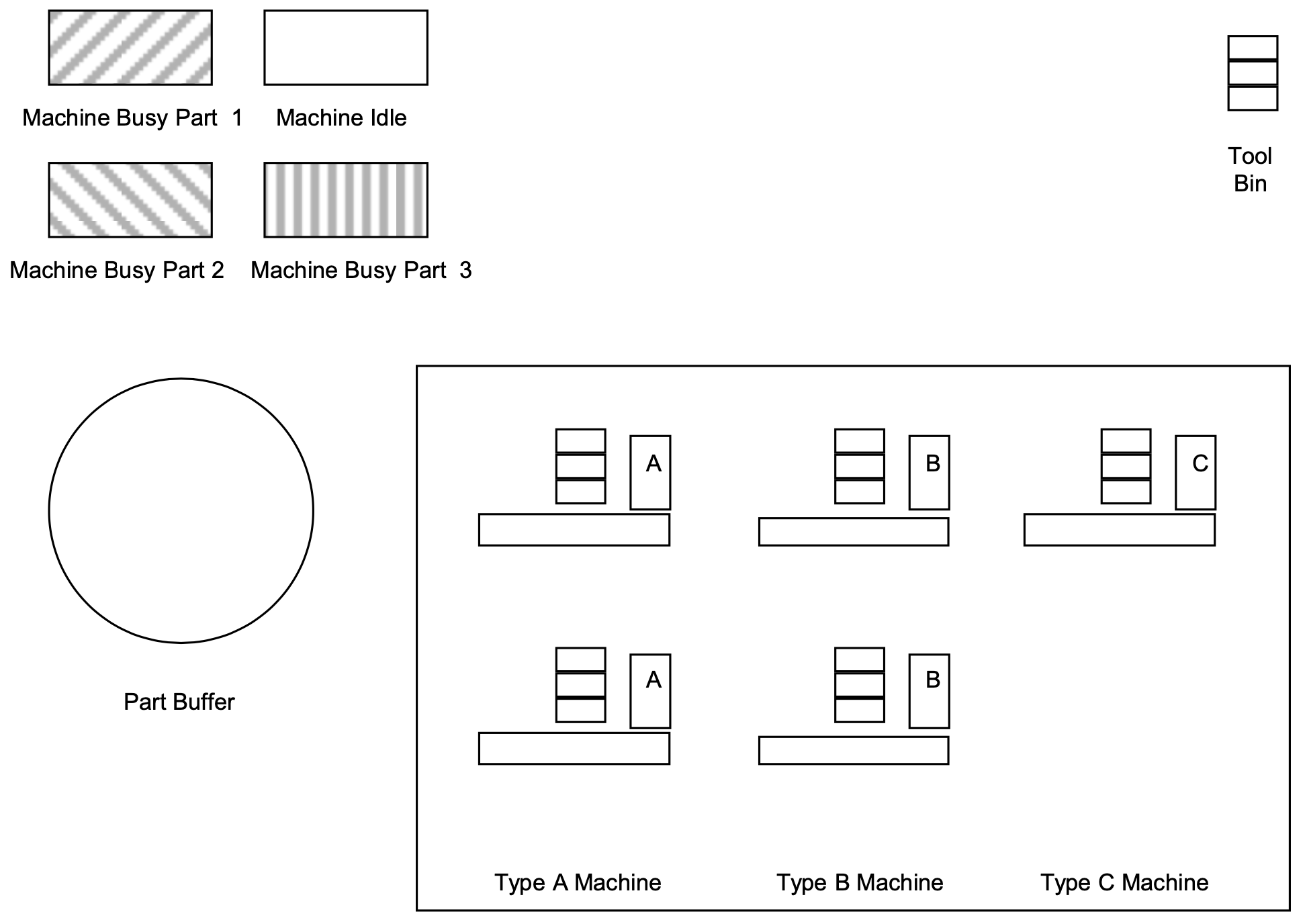
Figure 12-1 shows the system completely idle before a production run is made. Tool bins hold the tools currently assigned to each machine. The state of each machine, in terms of the type of part being processed, is shown. The system contains two type A machines, two type B machines, and one type C machine.
Production of 240 parts in one day is of interest. Parts arrive in batches of 24 every 75 minutes starting at the beginning of the day. The mix of part types in each batch is the same: 4 of type 1; 10 of type 2; and 10 of type.
Figure 12-1: Flexible Manufacturing System
Management wishes to minimize the makespan for the 240 parts as well as in-process inventory. Recall that the in-process inventory level is proportional to the number of fixtures and pallets the FMS requires. The lead time for parts in the FMS is of interest. The utilization of each machine is important.
Part and tool movement between machines requires 30 seconds. Machine setup time is minimal and can be ignored.
Table 12-1 presents the operation time data.
| Operation Time (Min) | ||||||
| Part Type | Parts to Produce / Day | Operation ID | Machine Type A | Machine Type B | Machine Type C | Tool |
| 1 | 40 | 1 | 12 | 11 | 10 | A |
| 2 | 13 | 15 | B | |||
| 3 | 14 | 14 | C | |||
| 2 | 100 | 1 | 2 | 4 | A | |
| 2 | 2 | 6 | 6 | C | ||
| 3 | 100 | 1 | 4 | D | ||
| 2 | 5 | 8 | E | |||
| 3 | 4 | F | ||||
12.3.1 Define the Issues and Solution Objective
The method for assigning a part operation, as well as the tool required by that operation to a machine, must be determined. Two schemes are proposed.
- Assign the part operation and tool to the IDLE machine with the shortest processing time for that operation at the time the part is ready to begin the operation. (Dynamic Scheduling).
- Assign each part operation to one and only one machine type using the machine loading heuristic in Askin and Standridge (1993), pp. 144-153.
Regardless of the scheme used, movement of parts and tools between machines will be minimized. The subsequent operation on a part will be performed on the same machine as the current operation if subsequent operation is allowed on that machine and the required tool is already loaded on the machine. Whether the same machine can perform the subsequent operation will be determined when the current operation is completed.
Note that the first scheme uses any machine that can perform the operation on a part. It selects between IDLE machines based on operation time, smallest time first. It seeks to avoid part waiting and to minimize the waiting time for each operation.
The second scheme seeks to balance the work load among the machines. It will make a part wait for its assigned machine type even if a machine of another type is IDLE and could process the part.
The priority order of machines for each operation on each part type using the dynamic scheduling approach with the machine having the shortest processing time given priority is shown in Table 12-2, which directly results from the data in Table 12-1.
| Part Type | Operation ID | First Priority | Second Priority | Third Priority |
| 1 | 1 | C | B | A |
| 2 | A | B | ||
| 3 | B | A | ||
| 2 | 1 | A | B | |
| 2 | A | C | B | |
| 3 | 1 | A | ||
| 2 | A | C | ||
| 3 | C |
The machine loading heuristic of scheme 2 seeks to equalize the workload between machine types. Results of applying the optimization algorithm to assign operations to machine types are given in Table 12-3.
| Part Type | Operation ID | First Priority | Second Priority | Third Priority |
| 1 | 1 | C | ||
| 2 | B | |||
| 3 | B | |||
| 2 | 1 | A | ||
| 2 | A | |||
| 3 | 1 | A | ||
| 2 | A | |||
| 3 | C |
Note the difference between the two schemes. The first priority machine type for each is the same, except for operation 2 on part type 1. In the first scheme, a part proceeds to a second or third priority machine if the first priority machine is busy. In the second scheme, a part simply waits if the first priority machine is busy.
12.3.2 Build Models
The model includes arrivals of batches of parts as well as decomposing the batches into individual parts. Thus, arriving entities represent batches of parts and subsequent entities represent parts. The part entities have the following attributes:
| ArrivalTime | = Time of arrival to the FMS |
| PartType | = Part type |
| Machine | = Machine used in current operation |
| Tool | = Tool used in current operation |
| OpTime | = Operation time for current operation = f(machine used) |
| CurrentOp | = ID number of the current operation (1, 2, 3) |
The model of an operation on a part requires two resources, one representing a machine and the other a tool. Movement between machines must be included in the model both for parts and tools. An procedure to select the machine to perform an operation on a part is included as well as a second procedure to determine whether the machine on which a part currently resides can perform the next operation.
Each tool resource has an attribute: ToolLocation = The machine on which it currently resides.
The pseudo code for the arrival process follows. A batch of 24 parts arrives every 75 minutes. Ten batches arrive in total. Each batch is separated into component parts: 4 of type 1, 10 of type 2, and 10 of type 3. Each part is sent to a process that models the first operation that is performed on it.
| Define Arrivals: \(\ \quad \quad\)Batches \(\ \quad \quad\quad\)Time of first arrival: \(\ \quad \quad\quad\)Time between arrivals: \(\ \quad \quad\quad\)Number of arrivals: |
0 75 minutes 10 |
| Define Resources: \(\ \quad \quad\)// Flexible Machine Resources \(\ \quad \quad\)MachA_1/1 \(\ \quad \quad\)MachA_2/1 \(\ \quad \quad\)MachB_1/1 \(\ \quad \quad\)MachB_2/1 \(\ \quad \quad\)MachC_1/1 // Tool Resources \(\ \quad \quad\)ToolA/1 \(\ \quad \quad\)ToolB/1 \(\ \quad \quad\)ToolC/1 \(\ \quad \quad\)ToolD/1 \(\ \quad \quad\)ToolE/1 \(\ \quad \quad\)ToolF/1 |
with states (Busy, Idle) with states (Busy, Idle) with states (Busy, Idle) with states (Busy, Idle) with states (Busy, Idle) with states (Busy, Idle) with states (Busy, Idle) with states (Busy, Idle) with states (Busy, Idle) with states (Busy, Idle) with states (Busy, Idle) |
| Define StateVariables: \(\ \quad \quad\)WIPCount \(\ \quad \quad\)ToolLocation(5) |
// Number of parts in FMS // Tool location |
| Define Lists: \(\ \quad \quad\)OpOneList OpTwoList \(\ \quad \quad\)OpThreeList |
|
| Define Entity Attributes: \(\ \quad \quad\)ArrivalTime \(\ \quad \quad\)PartType \(\ \quad \quad\)Machine \(\ \quad \quad\)Tool \(\ \quad \quad\)OpTime \(\ \quad \quad\)CurrentOp |
// Time of arrival to the FMS // Part type // Machine used in current operation // Tool used in current operation // Operation time for current operation = f(machine used) // ID number of the current operation (1, 2, 3) |
| Process BatchArrival Begin \(\ \quad \quad\)ArrivalTime = Clock \(\ \quad \quad\)CurrentOp = 1 \(\ \quad \quad\)PartType = 1 \(\ \quad \quad\)Clone 4 OpFirst \(\ \quad \quad\)PartType = 2 \(\ \quad \quad\)Clone 10 OpFirst \(\ \quad \quad\)PartType = 3 \(\ \quad \quad\)Clone 10 OpFirst End |
// arrival of a batch of 24 parts // type 1 parts // type 2 parts // type 3 parts |
Each part requires either two or three operations. The processes for each of the operations are similar but not identical. Each includes two essential steps: the transportation of the part and tool to the machine, if required, followed by the actual operation on the part. Two resources, a machine and a tool, are required. Which machine is determined by the machine assignment scheme employed.
At the beginning of the model of the first operation, the machine selection procedure is used to determine if the required tool is available. If so, the procedure determines if any machine is available to process the part and if so which one should be employed. The machine selection procedure is as follows:
MACHINE SELECTION PROCEDURE (OPERATION_NUMBER, PART_TYPE)
{
\(\ \quad \quad\)IF THE REQUIRED TOOL RESOURCE FOR THE PART_TYPE FOR
\(\ \quad \quad\)OPERATION_NUMBER IS IN THE IDLE STATE
\(\ \quad \quad\){
\(\ \quad \quad\quad\)FOR EACH MACHINE TYPE IN PRIORITY ORDER
\(\ \quad \quad\quad\){
\(\ \quad \quad\quad\quad\)IF ANY MACHINE OF THAT TYPE IS IN THE IDLE STATE
\(\ \quad \quad\quad\quad\){
\(\ \quad \quad\quad\quad\quad\)Machine = RESOURCE ID OF SELECTED MACHINE
\(\ \quad \quad\quad\quad\quad\)Tool = RESOURCE ID NUMBER OF REQUIRED TOOL
\(\ \quad \quad\quad\quad\quad\)OpTime = OPERATION TIME FOR PART FOR OPERATION_NUMBER
\(\ \quad \quad\quad\quad\quad\)RETURN
\(\ \quad \quad\quad\quad\)}
\(\ \quad \quad\quad\)}
\(\ \quad \quad\)}
}
If the required tool is not free or no machine is available to perform the operation, the part entity must wait in a buffer. There is one buffer in the model for each of the three operations. When a tool or machine resource becomes free, the model will search each buffer to find a part to process.
If the required tool and a machine are available to process the part, the tool and machine resources enter the busy state. Part entity attributes are assigned the name of the tool and machine as well as the process time for the operation on the selected machine. A time delay to move the tool and or part to the selected machine is incurred. The tool attribute recording its location (ToolLocation) is assigned the name of the selected machine. The operation is performed on the part. When the operation is completed, the tool resource enters the IDLE state. The lists of part entities waiting for operations 1, 2 or 3 are searched and the processing of another part is begun if possible.
The pseudo code modeling the first operation follows.
| Process OpFirst Begin WIPCount ++ MachineSelection (CurrentOp, PartType) If Machine is Null then Add entity to list Op1List Else Begin // Perform first operation Get Tool Get Machine ToolLocation (Tool) = Machine Wait for 30 seconds Wait for OpTime Free Tool SearchforNextPart End Send to OpSecond End |
// Add one to number of parts in FMS // Tool and part movement // Perform operation // Procedure to search all lists for next part to use tool |
The model of the second operation begins by determining if the part can remain on the same machine using the subsequent machine procedure. This will be the case if the machine is able to perform the operation and the tool required for that operation is available.
If the part cannot remain on the machine used for the first operation, the resource modeling this machine enters the idle state. The lists of part entities waiting for operations 1, 2 or 3 are searched and the processing of another part is begun if possible. The machine selection procedure is used to attempt to find a machine to process the part entity completing the first operation in the same way as was done for the first operation.
If the second operation can be performed on the same machine as the first, the tool resource for this operation enters the busy state, the operation is performed, and the tool resource enters the idle state. The lists of part entities waiting for operations 1, 2 or 3 are searched and the processing of another part is begun if possible. Type 2 parts do not require a third operation. Thus, at the end of the second operation, the machine resource processing a type 2 part enters the idle state and the search of the lists of waiting parts is conducted. The pseudo code for the second operation follows. The model of the third operation is similar to the model of the second operation.
SUBSEQUENT MACHINE PROCEDURE (OPERATION_NUMBER, PART_TYPE, CURRENT_MACHINE)
{
\(\ \quad \quad\)IF THE REQUIRED TOOL RESOURCE FOR OPERATION_NUMBER ON THIS PART IS
\(\ \quad \quad\)IN THE IDLE STATE
\(\ \quad \quad\){
\(\ \quad \quad\quad\)IF THE REQUIRED TOOL RESOURCE FOR OPERATION_NUMBER ON PART_TYPE
\(\ \quad \quad\quad\)IS LOADED ON CURRENT_MACHINE AND CURRENT_MACHINE CAN PERFORM
\(\ \quad \quad\quad\)OPERATION_NUMBER ON THIS PART_TYPE
\(\ \quad \quad\quad\){
\(\ \quad \quad\quad\quad\)THE REQUIRED TOOL RESOURCE ENTERS THE BUSY STATE
\(\ \quad \quad\quad\quad\)Tool = RESOURCE ID NUMBER OF REQUIRED TOOL
\(\ \quad \quad\quad\quad\)OpTime = OPERATION TIME FOR PART_TYPE FOR OPERATION_NUMBER
\(\ \quad \quad\quad\)}
\(\ \quad \quad\)}
}
| Process OpSecond Begin \(\ \quad\)CurrentOp = 2 \(\ \quad\)SubsequentMachine (CurrentOp, PartType, Machine) \(\ \quad\)If Tool is Null then \(\ \quad\)Begin \(\ \quad\quad\)// Move to another machine \(\ \quad\quad\)Free Machine \(\ \quad\quad\)SearchforNextPart \(\ \quad\quad\)MachineSelection (CurrentOp, PartType) \(\ \quad\quad\)If Machine is Null then Add entity to list Op2List \(\ \quad\quad\)Else \(\ \quad\quad\quad\)Begin \(\ \quad\quad\quad\quad\)// Perform second operation on another machine \(\ \quad\quad\quad\quad\)Get Tool \(\ \quad\quad\quad\quad\)Get Machine \(\ \quad\quad\quad\quad\)ToolLocation (Tool) = Machine \(\ \quad\quad\quad\quad\)Wait for 30 seconds \(\ \quad\quad\quad\quad\)Wait for OpTime \(\ \quad\quad\quad\quad\)Free Tool \(\ \quad\quad\quad\quad\)SearchforNextPart \(\ \quad\quad\quad\)End \(\ \quad\quad\)End \(\ \quad\quad\)Else \(\ \quad\quad\quad\)Begin \(\ \quad\quad\quad\quad\)// Perform second operation on current machine \(\ \quad\quad\quad\quad\)Get Tool \(\ \quad\quad\quad\quad\)Wait for OpTime \(\ \quad\quad\quad\quad\)Free Tool \(\ \quad\quad\quad\quad\)SearchforNextPart \(\ \quad\quad\quad\)End \(\ \quad\quad\)Send to OpThird End |
// Procedure to search all lists for next machine to use tool // Find another machine // Tool and part movement // Perform operation // Procedure to search all lists for next part to use tool // Perform operation // Procedure to search all lists for next part to use tool |
12.3.3 Identify Root Causes and Assess Initial Alternatives
The simulation experiment will determine both the makespan for 240 parts as well as the number of pallets and fixtures required. The latter can be accomplished by measuring the number of parts in the FMS as was previously discussed.
The design of the simulation experiment is summarized in Table 12-4. We are interested in the time to produce 240 parts. Thus, a terminating experiment with initial conditions of no parts in the system is appropriate. Since no quanities are modeled using probability distributions, no random number streams are needed and one replicate is sufficient. The two schemes for assigning parts to machines identified above are to be simulated. Performance measures have to do with the time to complete production on 240 parts, the lead time for parts, the number of parts in the FMS (WIP), and the utilization of the machines.
Results are shown in Table 12-5.
| Element of the Experiment | Values for This Experiment |
| Type of Experiment | Terminating |
| Model Parameters and Their Values | Machine load scheme used: 1. Available machine with the shortest processing time 2. Machine loading heuristic from Askin and Standridge |
| Performance Measures | 1. Time to produce 240 parts 2. Number of parts in the FMS (WIP) 3. Part Lead Time 4. Machine Utilization |
| Random Number Streams | None |
| Initial Conditions | Empty buffers and idle stations |
| Number of Replicates | 1 |
| Simulation End Time | Time to produce 240 parts |
| Loading Scheme | ||
| Performance Measure | Shortest Processing Time First | Balance Machine Type Workloads |
| Makespan (Minutes) | 1099 | 900 |
| WIP- \(\ \quad\quad\)Average \(\ \quad\quad\)Maximum |
30.8 63 |
46.2 86 |
| Lead Time (Minutes)- \(\ \quad\quad\)Average \(\ \quad\quad\)Standard deviation |
141 114 |
173 74 |
| Machine Utilization- \(\ \quad\quad\)Type A \(\ \quad\quad\)Type B \(\ \quad\quad\)Type C |
69.5% 72.5% 70.0% |
82.8% 67.5% 96.0% |
The makespan for the balance machine type workloads approach is 199 minutes less than for the shortest processing time first approach. The former approach results in higher utilizations for machine types A and C as well as a lower utilization for machine type B. Recall that operations were assigned to machine types A and C instead machine type B since the operation times for machine type B most often were higher than for the other two types.
Recall from the VUT equation that increasing the utilzation results in a longer lead time at a station. Thus, it could be expected that the balance machine type workloads approach would have a longer lead time than the shortest processing time first approach. In addition, Little's Law indicates that the WIP is proportional to the lead time and thus could also be larger. However, the balance machine type workloads scheme reduces the standard deviation of the lead time.
The maximum number of parts in the FMS is higher under the balance machine type workloads approach. This means that more fixtures and pallets are required using this approach.
12.3.4 Review and Extend Previous Work
Management accepted the simulation results presented in the previous section and decided to use the balance machine type workloads scheme. This decision was primarily based on the need to mimimize makespan. The cost of additional fixtures and pallets will be bourn to support this approach.
12.3.5 Implement the Selected Solution and Evaluate
During system operation, the time to produce a required batch of parts and the number of parts in the FMS will be monitored.