12.4: Summary

This case study shows how ad hoc operating rules, such as use the idle machine with the shortest processing time, are often inferior to operation rules developed using formal models. Simulation is used to test alternative rules and quantify the difference in their effects. Because systems are complex, simulation is needed even when such system operating models are deterministic. Complexity arises from the concurrent use of multiple resources such as tools and machines as well as the ability of resources such as machines to serve multiple tasks. The need for the model to organize and manage entities waiting for such resources instead of relying on the simulation engine to do so transparently to the model has been demonstrated.

Problems

1. Provide validation evidence for the FMS machine loading simulation based on the tool and machine utilization. Compute the expected utilization of each tool and machine type. Compare these results to the simulation results for the balance machine type workloads case. The machine utilization is shown in Table 12-5.

   Tool Utilization
   A	74.2%
   B	68.9%
   C	93.8%
   D	50.5%
   E	59.8%
   F	49.5%

2. Tell why the standard deviation of the time parts spend in the FMS (lead time) is greater than 0 since there are no random variables in the model.
3. Is it proper to compute a t-confidence interval for the mean part lead time? Why or why not?
4. Defend the use of the shortest processing time first loading scheme based on the simulation results shown in Table 12-5.
5. List service systems that you have encountered that have the flexibility characteristics of the manufacturing system discussed in this chapter.
6. Compare the model of the FMS to the model of the serial system discussed in chapter 7.
7. Write the model of third operation on a part in pseudo-code.
8. The model in this case study assumes that tools and parts can be moved concurrently to a machine. Modify the process model so that first the part is moved then the tool. Movements occur only if the part or tool is not resident on the selected machine.
9. Resimulate the model with all parts available for processing at time 0 and compare the results to those in Table 12-5.
10. Simulate the following improved version of the shortest processing time first rule and compare the results with those in Table 12-5. Don't allow operation 1 on machine type A.
11. Assess the effect of operation clustering on machine loading. Operations are assigned to specific machines, not just machine types. All part type 2 operations are assigned to one type A machine along with the first operation for part type 3. The second operation for part type 3 is assigned to the other A machine. The third operation for part type 3 is assigned to the type C machine. The first operation for part type 1 is assigned to the type C machine, the second to one type B machine, and the third to the other type C machine.
12. Develop and test heuristics that embellish the operation clustering based assignment given in the previous problem. For example, allow the least utilized machine to be a second priority for the most utilized machine if feasible.
13. Management will purchase one more tool of any of the six tool types if that will help shorten makespan. Which tool should be purchased? Evaluate your choice using the simulation model developed in this chapter.
14. Test the idea that a part should stay on the same machine as long as it is feasible for that machine to perform the next operation on the part. In this case, the required tool is moved to that machine as soon as it is idle.

Case Problem

A flexible manufacturing facility must produce 1680 parts of one type per 80-hour lead (Wortman and Wilson, 1984; Kleijnen and Standridge, 1988). The part flow through the facility is follows.

1. Parts arrive to the facility from a lathe at a constant rate of 21 per hour.
2. Parts require three operations in the following sequence: Op10, Op20, and Op30.
3. A part is washed before and after each operation.

Each operation is performed either by a fixed machine or a flexible machine. A fixed machine can perform one and only one of three operations but a flexible machine can perform any of the three operations. Parts are moved between machines and the wash station by a single automated guided vehicle (AGV). The AGV system transports parts with little or no human assistance. The vehicle picks up loads at designated pick-up points and transports them to designated drop-off points. Each pick-up and drop-off point is associated with a machine or work station. A central computer assigns material movement tasks to the AGV and monitors the vehicle position. The AGV moves in one direction on a fixed track around the center of the system.

Operation processing times are 14.0, 5.0, and 8.0 minutes respectively for Op10, Op20, and Op30. Washing time is 18 seconds.

AGV travel time is 20 seconds around the entire loop. The following table shows AGV travel time between each pair of workstations.

	Wash Station	OP 10	OP 20	OP 30	Flexibile
Wash Station	0	5	9	15	11
OP10	5	0	4	10	6
OP20	9	4	0	15	11
OP30	15	10	15	0	16
Flexible	11	6	11	16	0

Figure 12-2 gives an overview of the system at the beginning of the production period with all machines idle and no parts in the system. Part movement by the AGV is indicated. The particular operation performed by each machine is displayed.

Figure 12-2: Overview of the Flexible Manufacturing System: (4, 2, 2, 1) Configuration.

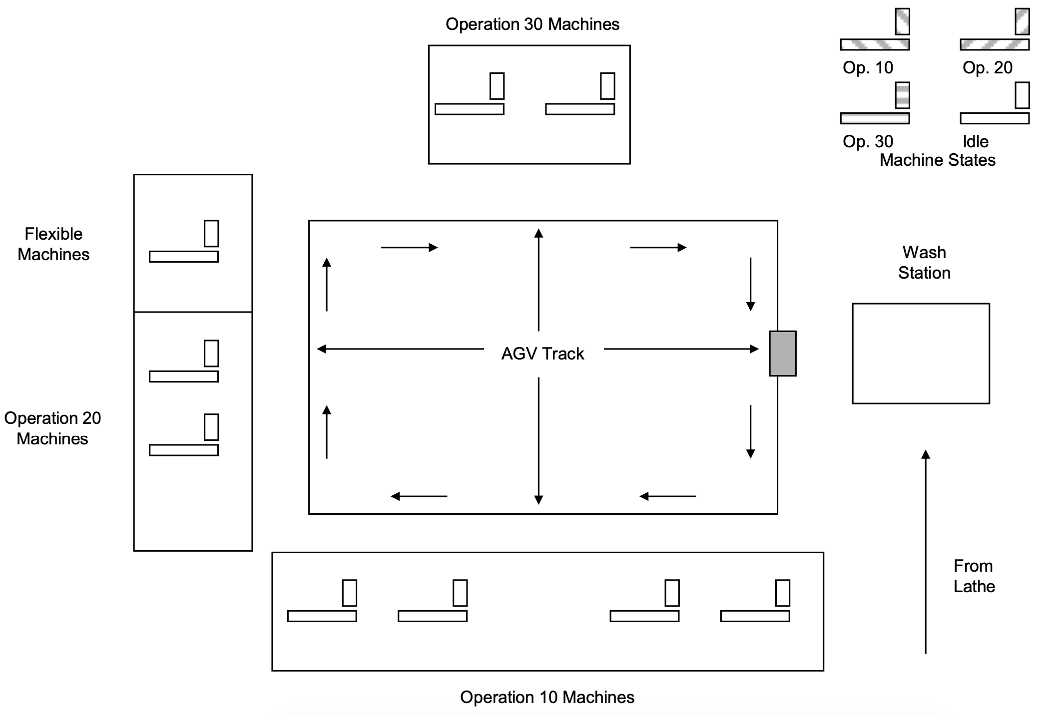
The objective is to find the minimum cost combination of fixed machines (Op10, Op20, or Op30 only) and flexible machines (all three operations) that meets the throughput requirement. Flexible machines cost more than fixed machines. Thus, all possible work should be done by fixed machines. Flexible machines are employed to avoid buying an excessive number of fixed machines. In addition, management is also interested in minimizing lead time for a part. Thus, management will consider a configuration of machines that includes flexible machines and increases cost in order to reduce lead time as long as the total number of machines does not exceed the total number of fixed machines required to do the work by more than one.

The following operating rule is employed for each operation to select between fixed and flexible machines. A part will use a fixed machine if it is available. If not, it will use a flexible machine if one is available. If neither a fixed machine nor a flexible machine is available, the part will use the first machine of either type, fixed or flexible, that becomes available.

One possibility that should be considered is using the minimum number of fixed machines needed to process all parts in a timely fashion with no flexible machines utilized.

Assess the structural variability seen in this system. Generate a trace of all system activities. Use the trace to identify the structural variability.

Case Problem Issues

1. What performance measure are important in this problem?
2. How will the AGV system be modeled?
3. Describe how to model the choice between a fixed and a flexible machine for an operation in the simulation language you are using.
4. When does a part entity acquire and free a machine resource relative to acquiring and freeing the AGV resource?
5. How can the effect on system operations of part waiting for the AGV be determined.
6. How many fixed machines of each type are needed if no flexible machines are used?
7. Construct an alternative to the machine configuration in number 6 as follows. Replace one fixed machine of each type with a sufficient number of flexible machines. Determine the number of flexible machines in this case.
8. Why tell why all parts do not have the same time in the system.