13.3: The Case Study

A large manufacturer of office supplies (pens, pencils, tape, etc.) sells in large volume to a discount office supply retailer. In order to retain this customer, the manufacturer must manage the customer's inventory and automatically generate shipments of products when necessary. Missing any shipment due to a lack of available product results in a large financial penalty. However, management wishes to minimize the amount of inventory on hand to keep storage space costs and investment in unsold product low. In addition, it is in the best interest of the manufacturer if the retailer does not lose any sales due to a lack of product on hand. At the same time, the manufacturer cannot expect the retailer to keep excessive inventory.

13.3.1 Define the Issues and Solution Objective

We will consider only one product. Others can be assessed in a similar manner. Sales data supplied by the customer can be analyzed and the daily sales volume characterized by a statistical distribution. The sales data concerns one region with 37 stores. Thus, this data is a sum of 37 values. As was discussed in Chapter 5, the normal distribution may provide a good fit to such data. Using software for fitting data to distributions, it was found that a normal distribution with mean 180 cartons and standard deviation 30 cartons fits the actual daily regional sales data.

The manufacturer and the retailer have agreed that one shipment every three days on the average is acceptable. The distribution of three days sales can be determined using probability theory as follows. The distribution of the sum of three normally distributed random variables is also normally distributed with the mean equal to the sum of the three means and variance equal to the sum of the three variances. (Standard deviations don't add.) Thus, three days sales is normally distributed with mean 540 cartons and standard deviation 52 cartons. The 99% percent point of normal distribution with mean 540 and standard deviation 52 is approximately 660. Thus, the amount of inventory needed to meet three days of sales with probability 99% is 660 cartons.

The reorder point, the inventory level that triggers a shipment from the manufacturer, must be set. Since shipments take one day, it is tempting to set the reorder point to the amount of inventory to meet one day's demand with probability of 99%, approximately 250 cartons. However, consider the consequences if the inventory at the end of a day is 300 cartons. No shipment is sent. The next day suppose the demand is 120 cartons leaving 180 cartons in inventory and triggering a shipment. The probability of the following day's demand exceeding 180 cartons is 50%. Thus, sales could be lost while the shipment is being processed.

The reorder point will be set at the amount of inventory to meet two days demand with probability of 99%. Two days demand is normally distributed with mean 360 and standard deviation 42. Thus the reorder point is set to be 460 cartons.

The nominal maximum production level for the product is 240 cartons per day. Actual data shows the production level to be uniformly distributed between 220 and 235 due to units that fail to pass inspection and random equipment failures.

There is no production on any day if inventory at the manufacturer is sufficiently high to meet the next shipment. A range for this inventory level, called the production cut-off point, can be computed as follows. The target number of units in inventory at the retailer after a shipment is received is 660. An order, which takes one day to receive, is placed when there are 460 cartons in inventory. The average number of sales in one day is 180 cartons. Thus, the average shipment has (660 - 460) + 180 = 380 cartons. The maximum shipment to the retailer is 660 cartons.

There are two important parameters of the inventory system:

1. The number of cartons in the inventory of the retailer, the reorder point, that triggers a new shipment from the manufacturer, currently proposed to be 460 cartons.
2. The number of cartons in inventory at the manufacturer that allows the following day's production to be canceled, the production cut-off point, currently proposed to be in the range 380 to 660 cartons.

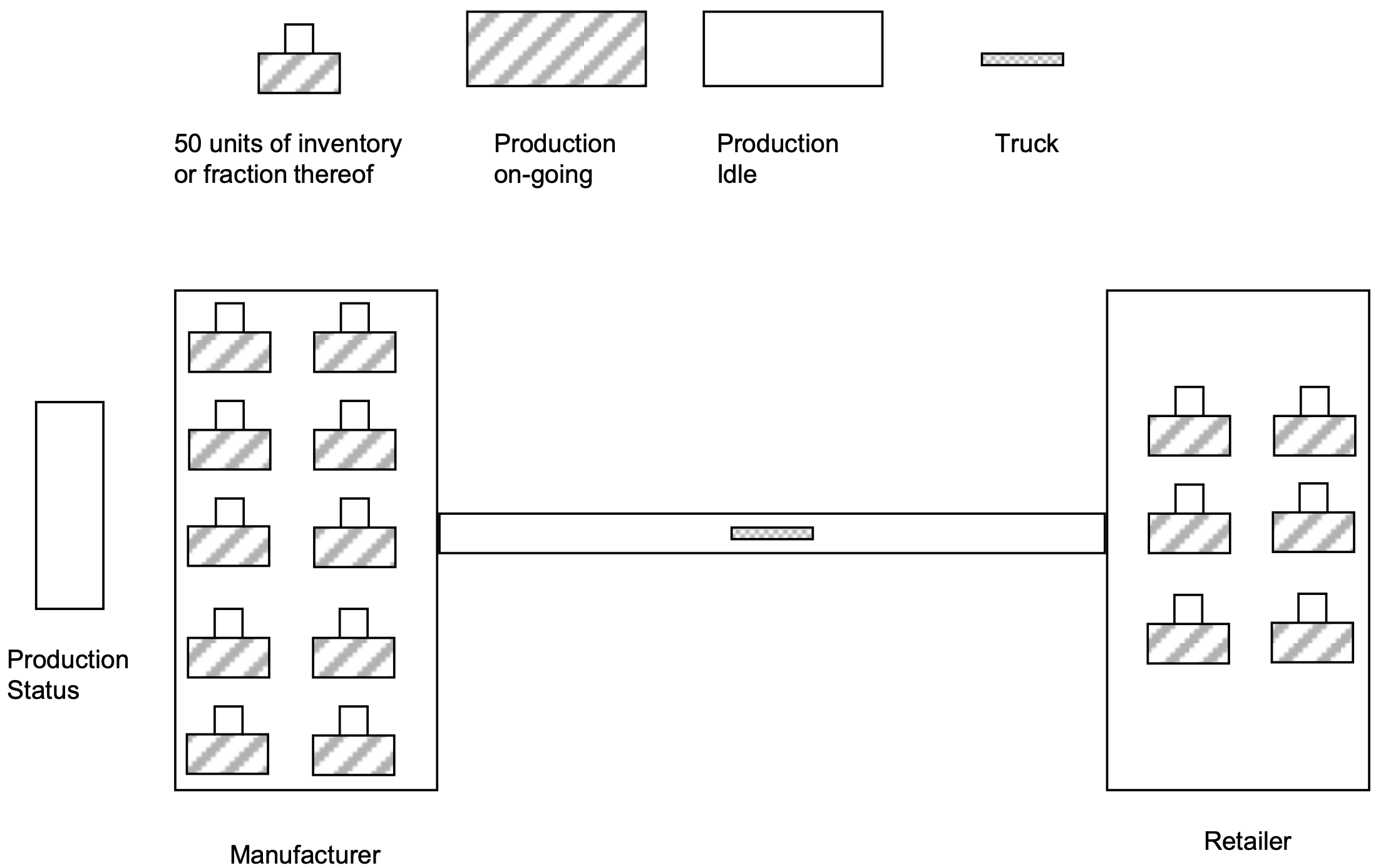
Figure 13-1 summarizes the inventory system. Inventory is generated by production at the manufacturer and moved to the retailer as needed. Inventory levels, product movement, and production status are shown. Note again how this system is driven by dynamic decisions based on the values of state variables.

Figure 13-1: Automated Inventory Management System

13.3.2 Build Models

The model consists of three parallel processes:

1. Production at the manufacturer.
2. Sales at the retailer.
3. Shipments from the manufacturer to the retailer.

The first two processes schedule entity arrivals every day. The latter processes event triggered arrivals that occur when the retailers inventory drops below 460 cartons.
First the variables used throughout the model will be defined.

---

Define Variables ProductionInv RetailInv Cutoff DailyProd Sold Demand Reorder Ordered Shipped

// Amount of inventory at the manufacturing plant // Amount of inventory at the retail plant // Production cut off level // Daily production at the manufacturing facility // Daily sales // Daily demand // Reorder Point // Order volume from retailer // Number of units shipped from the manufacturing

---

Consider production at the manufacturer. A entity arrives once per day to control the production of new units. If the number of units in inventory is less than the production cut-off point, new units are made and added to the inventory. The model of this process follows.

---

Define Arrivals:
\(\ \quad \quad\)Time of first arrival: 0
\(\ \quad \quad\)Time between arrivals: 1 day
\(\ \quad \quad\)Number of arrivals: Infinite

Process Manufacture
Begin
\(\ \quad \quad\)If ProductionInv > CutOff then
\(\ \quad \quad\)Begin // No need for production today
\(\ \quad \quad\quad\)Tabulate 0 in Production
\(\ \quad \quad\)End
\(\ \quad \quad\)Else
\(\ \quad \quad\)Begin // Produce today
\(\ \quad \quad\quad\)Tabulate 100 in T_Production
\(\ \quad \quad\quad\)Set DailyProd = uniform 220, 235
\(\ \quad \quad\quad\)Increment ProductionInv by DailyProd
\(\ \quad \quad\)end
End

---

Next consider the process for sales at the retailer. One entity representing sales information is created each day. The number of units demanded may exceed those available in inventory. This is an undesirable situation. The number of units demanded beyond those that are available in inventory represents lost sales. The model of the sales process follows.

Final consider the order process. A state event occurs when the number of units in the retail inventory becomes less than 460. The time till delivery is one day. The ordering process follows.

---

Define Arrivals:
\(\ \quad \quad\)Time of first arrival: 0
\(\ \quad \quad\)Time between arrivals: 1 day
\(\ \quad \quad\)Number of arrivals: Infinite

Process Sales
Begin
\(\ \quad \quad\)Set Demand = normal 180, 30
\(\ \quad \quad\)If RetailInv > Demand then
\(\ \quad \quad\)Begin // Sufficient Inventory to meet demand
\(\ \quad \quad\quad\)Tabulate 100 in DailySales
\(\ \quad \quad\quad\)Set Sold = Demand
\(\ \quad \quad\)End
\(\ \quad \quad\)Else
\(\ \quad \quad\)Begin // Insufficient Inventory to meet demand
\(\ \quad \quad\quad\)Tabulate 0 in DailySales
\(\ \quad \quad\quad\)Set Sold = RetailInv
\(\ \quad \quad\)End

\(\ \quad \quad\)Decrement RetailInv current by Sold
End

---

---

Define Arrivals:
\(\ \quad \quad\)When RetailInv becomes less than Reorder
\(\ \quad \quad\)Number of arrivals: Infinite
Process Ship
Begin
\(\ \quad \quad\)Set Ordered = min (660, 660 - RetailInv + 180)

\(\ \quad \quad\)If Ordered > ProductionInv then
\(\ \quad \quad\quad \quad\)Begin // Insufficient inventory for today's order
\(\ \quad \quad\quad \quad\)Tabulate 0 in Shipments
\(\ \quad \quad\quad \quad\)Set Shipped = ProductionInv
\(\ \quad \quad\quad \quad\)End
\(\ \quad \quad\)Else
\(\ \quad \quad\)Begin // Sufficient Inventory
\(\ \quad \quad\quad \quad\)Tabulate 100 in Shipments
\(\ \quad \quad\quad \quad\)Set Shipped = Ordered
\(\ \quad \quad\)End
\(\ \quad \quad\)// Make shipment
\(\ \quad \quad\)Decrement ProductionInv by Shipped
\(\ \quad \quad\)Wait for 24 hr
\(\ \quad \quad\)Increment RetailInv by Shipped
End

---

13.3.3 Identify Root Causes and Assess Initial Alternatives

Table 13-1 gives the experiment design for the inventory system simulation.

Table 13-1: Simulation Experiment Design for the Inventory System

Element of the Experiment	Values for This Experiment
Type of Experiment	Terminating
Model Parameters and Their Values	1. Re-order point for retailers inventory, 460 units 2. Production cancellation point based on manufacturer's inventory (380, 660) units
Performance Measures	1. Number of days with lost sales 2. Amount of inventory at the retailer 3. Number of days with no production 4. Amount of inventory at the manufacturer 5. Number of shipments 6. Number of shipments with insufficient units
Random Number Streams	1. Number of units manufactured 2. Number of units demanded
Initial Conditions	1. Inventory at the retailer - average of the reorder point and the maximum desirable inventory, 560 units 2. Inventory at the manufacturer -- Mid-point of the product cancellation range, 520 units
Number of Replicates	20
Simulation End Time	365 days (one year)

Management felt that demand data would be valid for no more than one year. Thus, a terminating experiment with a time period of one year was used. The number of units demanded each day and the number of units produced each day that production occurs are modeled as random variables. Thus, two random number streams are needed. Twenty replicates will be performed.

The initial inventory at the manufacturer and at the retailer must be set. Management believed that typical conditions are as follows. The number of units at the retailer should most often be between the re-order point and the intended maximum inventory level or 460 - 660. The average of these values, 560, will be used for the initial conditions. A typical number of units at the manufacturer should be within the range of the cut-off level for production, 380 - 660 units. The mid-point of the range, 520, is used.

As discussed previously, model parameters are the re-order point for the retailers inventory, whose value in the first experiment will be 460 units, and the production cancellation point. The values used for this latter quantity are the average shipment size, 380 units, and the maximum shipment size, 660 units.

There are several performance measures. The number of days with lost sales measures how well the inventory management system helps the retailer meet demand for the product. In addition, the inventory level at the retailer is of concern. At the manufacturer, the number of days without production and the inventory level are of interest. Finally, the total number of shipments from the manufacturer to the retailer, as well as the number of shipments with less than the requested number of units, should be estimated. The latter results from a lack of inventory at the manufacturer.

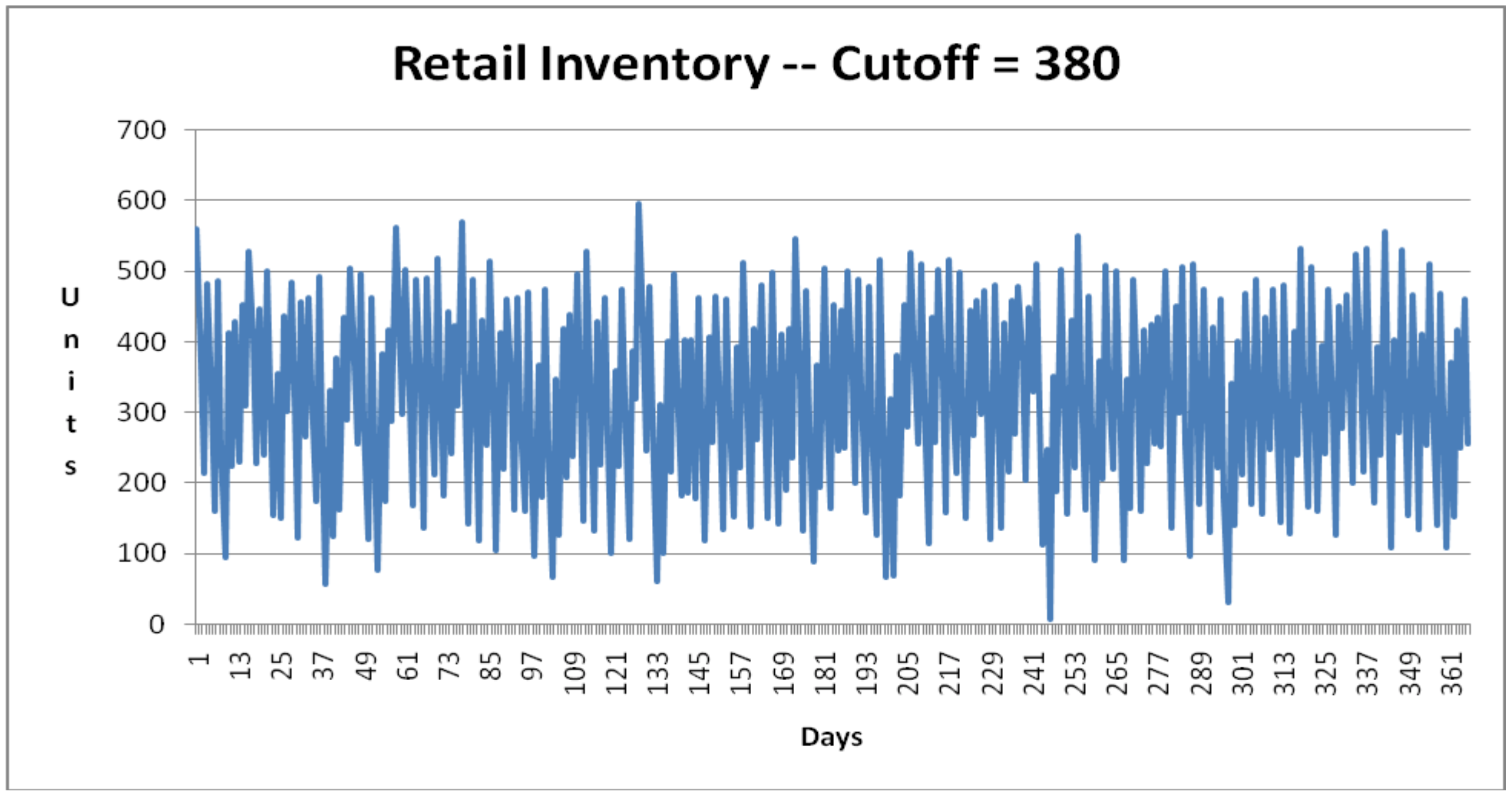
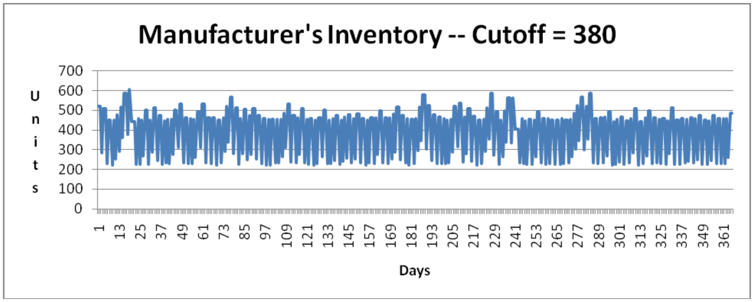
The inventory level at the retailer must be examined. Figures 13-2 and 13-3 show the inventory level at the retailer over time from the first replicate for each value of the cut-off point. In both graphs, the majority of the values are between 100 and 500 cartons.

Figure 13-2: Inventory at Retailer – Production Cut-off Point of 660

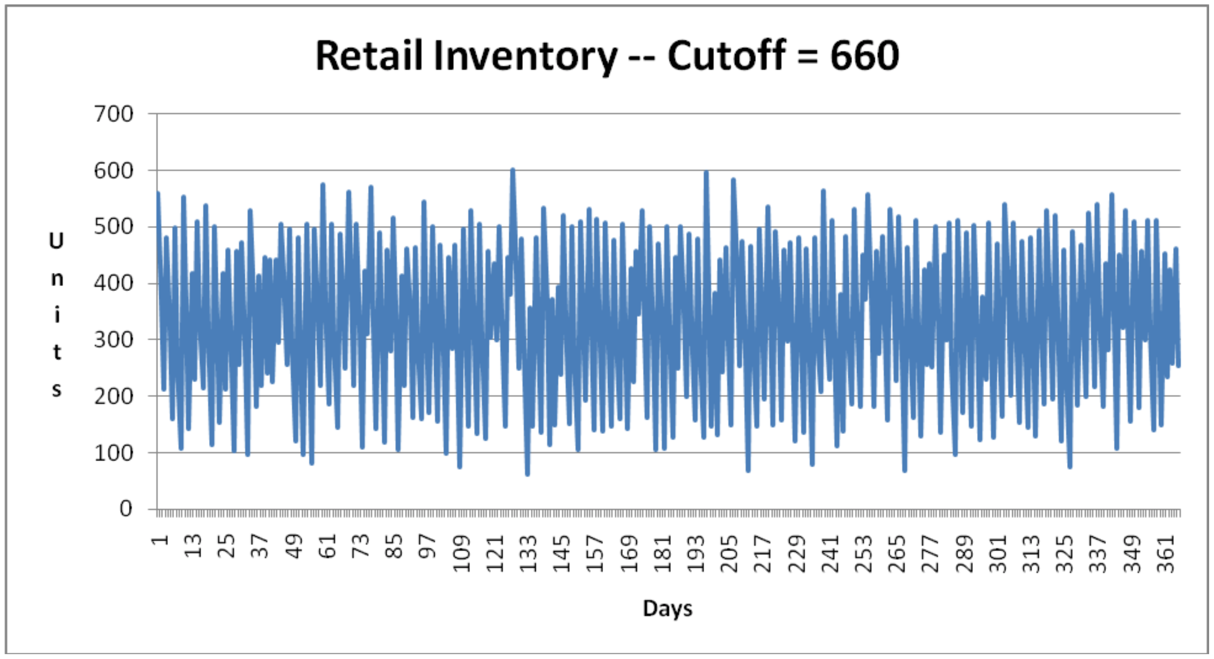
Figure 13-3: Inventory at Retailer – Production Cut-off Point of 380

Figures 13-4 and 13-5 show the inventory levels at the manufacturer for each value of the production cut-off point. The higher cut-off value, 660, results in an inventory between 400 and 800 cartons most of the time. The lower value, 380, results in an inventory between 200 and 500 cartons most of the time.

Figure 13-4: Inventory at Manufacturer – Production Cut-off Point of 660

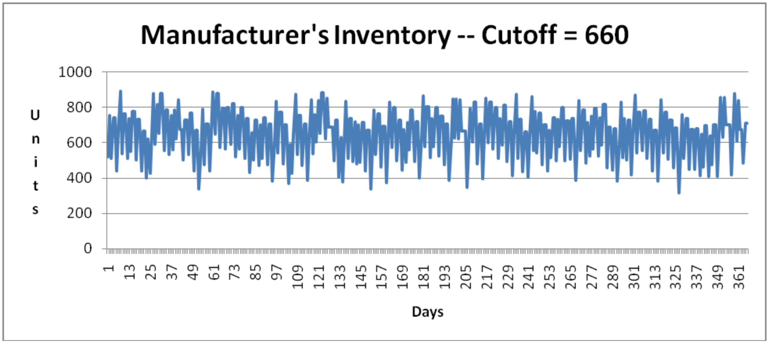
Figure 13-5: Inventory at Manufacturer – Production Cut-off Point of 380

There were only 4 days of lost sales over all 20 replicates when the cut-off point was 660 and 3 days when the cut-off point was 380. This indicates that the reorder point was set correctly, or at least not too low.

Table 13-2 summarizes the other performance measure values resulting from the simulation experiment.

The number of days with no production is approximately the same for both values of the production cut-off point. The number of days per year without production is about 78 or 1.5 days per week. Thus, 5.5 days of production per week should be sufficient.

When the higher production cut-off point is used, all shipments contain the number of units requested by the retailer. When the lower cut-off point is used, slightly less than half of the shipments have an insufficient number of units, that is fewer units than requested by the retailer. The lower cut-off value leads to an average of 10.4 additional shipments per year.

Table 13-2: Results of the Inventory System Experiment

	Days with No Production			# of Insufficient Shipments			Total # of Shipments
Replicate	Cut- off Point 660	Cut- off Point 380	Difference	Cut- off Point 660	Cut- off Point 380	Difference	Cut- off Point 660	Cut- off Point 380	Difference
1	80	81	1	0	73	73	133	143	10
2	75	76	1	0	66	66	137	147	10
3	74	75	1	0	76	76	136	146	10
4	79	80	1	0	64	64	135	145	10
5	79	80	1	0	79	79	132	144	12
6	73	74	1	0	78	78	136	146	10
7	76	77	1	0	65	65	133	145	12
8	76	77	1	0	57	57	136	146	10
9	76	77	1	0	60	60	135	146	11
10	78	79	1	0	79	79	134	144	10
11	75	77	2	0	68	68	134	147	13
12	72	74	2	0	60	60	138	148	10
13	74	75	1	0	55	55	135	147	12
14	78	79	1	0	67	67	136	145	9
15	72	74	2	0	74	74	137	148	11
16	74	75	1	0	71	71	138	146	8
17	78	79	1	0	73	73	134	146	12
18	81	82	1	0	72	72	135	144	9
19	72	73	1	0	61	61	137	148	11
20	77	78	1	0	76	76	137	145	8
Average	75.9	77.1	1.2	0	68.7	68.7	135.4	145.8	10.4
Std. Dev.	2.7	2.6	0.4	0	7.5	7.5	1.7	1.4	1.4
99% CI Lower Bound	74.2	75.4	0.9	0	63.9	63.9	134.3	144.9	9.5
99% CI Upper Bound	77.7	78.8	1.4	0	73.5	73.5	136.5	146.7	11.3

13.3.4 Review and Extend Previous Work

Management felt that the foremost objective is to satisfy the retailer. The automated inventory management system appears to meet the objective. The retailer is able to meet all customer demand without carrying excessive inventory. Most of the time, the inventory is less than three days average demand for the product.

The higher value for the cut-off point is preferred. This results in no shipments with less units than the retailer demanded as well as fewer total shipments. Management is willing to accept a larger inventory at the manufacturer to better satisfy the customer.

Management noted that the variance between replicates is small. This small variance should make the automated inventory system easier to operate and control.

Production of the product 5.5 days a week will be scheduled.

13.3.5 Implement the Selected Solution and Evaluate

The automated inventory system will be installed and will operate with a reorder point of 460 units and a production cut-off point of 660 units. The retailer was assured by the simulation results of the ability to meet customer demand completely and consistently as well as holding a relatively low inventory. System performance will be monitored using the measures defined for the simulation experiment.