
13.4: Summary
- Page ID
- 31016

This chapter illustrates how dynamic decision making based on state variables may be incorporated into models. System details are not modeled directly. Aggregate behavior is modeled using statistical distributions. Graphs show the dynamics of inventory levels. System behavior due to alternative values of inventory system parameters is assessed.
Problems
- Provide verification evidence for the inventory system experiment based on the following results.
Number of days processed: 365 Number of days without production: 77 Number of days with production: 288 Number of shipments: 145 Number of shipments of sufficient quantity: 78 Number of shipments of insufficient quantity: 67 - Provide validation evidence for the inventory system experiment based on the simulation results presented in this case study.
- One possibility that could arise during the simulation experiment is the following. Suppose a shipment of insufficient units failed to bring the inventory at the retailer above the reorder point. What would be the consequences for the simulation experiment? What conclusions could be drawn about operating the system with the particular reorder and cut-off point values?
- Discuss management's decision to use the higher cut-off point value. Defend using the lower value since the customer can still meet all demand.
- Include detection and response of the condition described in problem 3 in the model and resimulate the using the lower value of the cut-off point.
- Find a cut-off point value between 380 and 660 that improves system operation. Use a reorder point of 460 units.
- Find a reorder point lower than 460 units that either improves system operation or makes it no worse.
- Print out a trace of the inventory at the retailer. For each day, include the inventory at the start of the day, the deliveries, the demand, and the inventory at the end of the day.
- Modify the model so that product occurs Monday through Friday at the current rate and Saturday at half the current rate. This implements the conclusion of the analysis that 5.5 days per week production on the average is sufficient. At the same time, customer demand at the retailer occurs 7 days per week. Would you expect more or less inventory to be needed at the retailer? Defend your expectation.
Case Problem
A product inventory changes daily due to customer demand that withdraws from it and production that replenishes it on the days when it is operating. Customer demands and production are random variables. Production is subject to down times of random frequency and duration. Customers due not backorder. Thus, any customer demand that cannot be met results in a lost sale.
Periodically, an analyst can review the inventory and make adjustments by purchasing or selling product on the spot market. The time between these reviews is called the review period. At each review, the analyst can do the following:
- If the current inventory is less than the safety stock, buy a quantity of product equal to (safety stock - current inventory) on the spot market.
- If the current inventory is greater than the maximum inventory, sell a quantity of product equal to (current inventory - maximum inventory) on the spot market.
The safety stock level is an operating parameter of the inventory system set such that the probability of meeting all customer demand between periodic reviews is at least a specified value, typically 90%, 95%, or 99%. This probability is called the effective service level.
The maximum inventory level is less that the physical limit on inventory storage, called the capacity, to avoid having no place to store items.
Figure 13-6 summarizes the inventory control system. Note the following definitions and notation.
Figure 13-6: Inventory Management System Summary
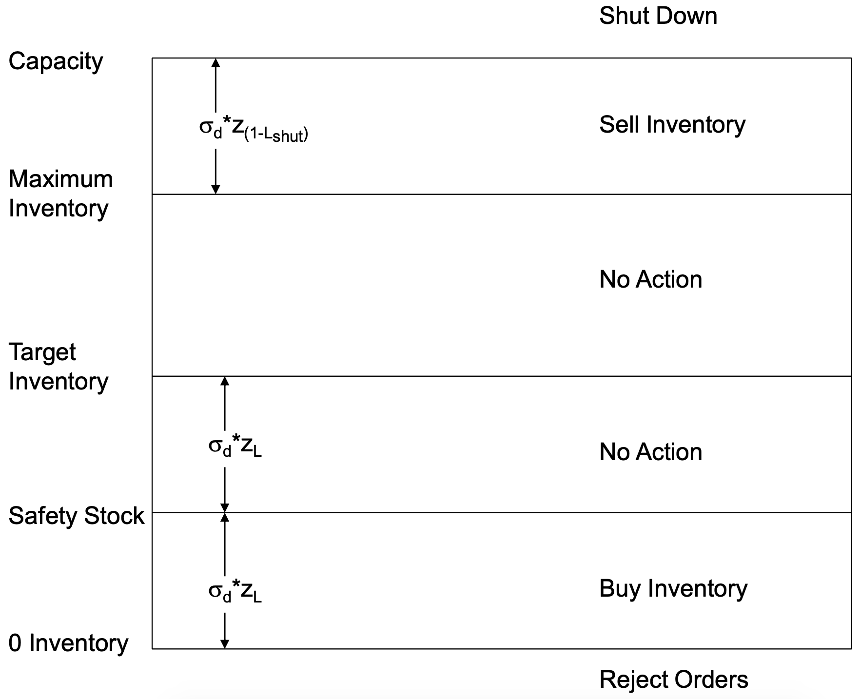
Target inventory - The desired inventory to avoid purchases and sales on the spot market, in the range [safety stock, maximum inventory].
Delta inventory - The change in inventory each day due to production (+) and demand (-).
Nominal service level - The probability that the inventory will be greater than the safety stock at the time of a review given that it was equal to the target at the time of the last review. As well, the probability that the inventory will be greater than zero at the time of a review given that it was equal to the safety stock at the time of the last review.
d = number of days in the review period
\( \mu_{\mathrm{d}}\) = the mean of the delta inventory distribution for a review period of d days
\(\ \sigma_{d}^{2}\)= the variance of the delta inventory distribution for a review period of d days
\(\ \mu_{p}\)= the mean of the conditional daily production distribution (given that production is greater than zero).
\(\ \sigma_{p}^{2}\)= the variance of the daily production distribution
\(\ \mu_{\mathrm{c}}\)= the mean of the daily customer demand distribution
\(\ \sigma_{\mathrm{c}}^{2}\)= the variance of the daily customer demand
A = the percent of days that production occurs (the availability of production)
L = the nominal service level as a percent
Leff = the effective service level
\(\ L=1-\sqrt{\left(1-L_{e f f}\right)}\)
Lshut = the probability of exceeding the capacity during the next review period given that the inventory level is equal to the maximum inventory at the current review
zL = The L% point of the standard normal distribution
The average demand is equal to the average production over a long period of time such as a year. This means that \(\ \mu_{c}=\mu_{p} * A\). In other words, the expected production each day (including an allowance for down time) is equal to the expected daily demand.
Ignoring down times, the delta inventory can be viewed approximately normally distributed with parameters:
\(\ \mu_{d}=0\)
\(\ \sigma_{d}^{2}=\sum_{i=0}^{d}\left[\sigma_{p}^{2}+\sigma_{c}^{2}\right]=d *\left[\sigma_{p}^{2}+\sigma_{c}^{2}\right]\)
The problem is to determine the review period, safety stock, maximum inventory, and target inventory given an effective service level. Performance measures should include the service level as well as the number of purchases and sales made to the spot market by the analyst.
Consider the following specifications.
| Capacity: | 10,000. |
| Distribution of customer demand: | Normal (1000, 250). |
| Distribution of production when production occurs: | Normal(1000/A, 300). |
| A=Availability: | 30/(30+1.92) |
| Review period: | 7, 10, or 14 days. |
| Effective service level: | 0.95 or 0.99. |
First, determine the required quantities assuming that there is no production downtime. Use analytic models to compute the safety stock, target inventory, and maximum inventory for each review period. Use simulation to validate the analytic computations. Make adjustments to the analytically computed quantities if necessary. Validate your final recommendation using simulation. Validate means to show that the required effective service level is met.
Next, consider production downtime. Establish and validate quantities for the safety stock, target inventory, and maximum inventory using simulation. The average time between periods of no production is 30 days. The average length of each period of no production is 1.92 days. The distribution of the period of no production follows.
Distribution of the Length of Periods of No Production
| Days down | Percent |
| 1 | 50% |
| 2 | 25% |
| 3 | 13% |
| 4 | 7% |
| 5 | 5% |
| Total | 100% |
Case Problem Issues
- Identify the processes that are needed in the model.
- Specify all of the combination of the values of the parameters that should be simulated.
- Compute the safety stock, target inventory level, and maximum inventory level for each parameter value combination using a spreadsheet.
- Specify the initial conditions for the simulation.
- In addition to service level, define the performance measures.
- Determine how production downtime should be modeled.
- Discuss how verification and validation evidence will be obtained.
The time period of interest is one year.