15.2: Points Made in the Case Study

Last updated
Save as PDF

Page ID: 31022

\( \newcommand{\vecs}[1]{\overset { \scriptstyle \rightharpoonup} {\mathbf{#1}} } \) \( \newcommand{\vecd}[1]{\overset{-\!-\!\rightharpoonup}{\vphantom{a}\smash {#1}}} \)\(\newcommand{\id}{\mathrm{id}}\) \( \newcommand{\Span}{\mathrm{span}}\) \( \newcommand{\kernel}{\mathrm{null}\,}\) \( \newcommand{\range}{\mathrm{range}\,}\) \( \newcommand{\RealPart}{\mathrm{Re}}\) \( \newcommand{\ImaginaryPart}{\mathrm{Im}}\) \( \newcommand{\Argument}{\mathrm{Arg}}\) \( \newcommand{\norm}[1]{\| #1 \|}\) \( \newcommand{\inner}[2]{\langle #1, #2 \rangle}\) \( \newcommand{\Span}{\mathrm{span}}\) \(\newcommand{\id}{\mathrm{id}}\) \( \newcommand{\Span}{\mathrm{span}}\) \( \newcommand{\kernel}{\mathrm{null}\,}\) \( \newcommand{\range}{\mathrm{range}\,}\) \( \newcommand{\RealPart}{\mathrm{Re}}\) \( \newcommand{\ImaginaryPart}{\mathrm{Im}}\) \( \newcommand{\Argument}{\mathrm{Arg}}\) \( \newcommand{\norm}[1]{\| #1 \|}\) \( \newcommand{\inner}[2]{\langle #1, #2 \rangle}\) \( \newcommand{\Span}{\mathrm{span}}\)\(\newcommand{\AA}{\unicode[.8,0]{x212B}}\)

In previous chapters, emphasis has been placed on one aspect of the operation of a system. Modeling an integrated supply chain requires integrating many components in one model: shipments, inventory management, customer demand, production, and information flow. Simulation has a unique ability to provide such integration. A model integrating these components is illustrated in this case study.

Work - Beyond Lean_ Simulation in Practice Second Edition-243.jpg

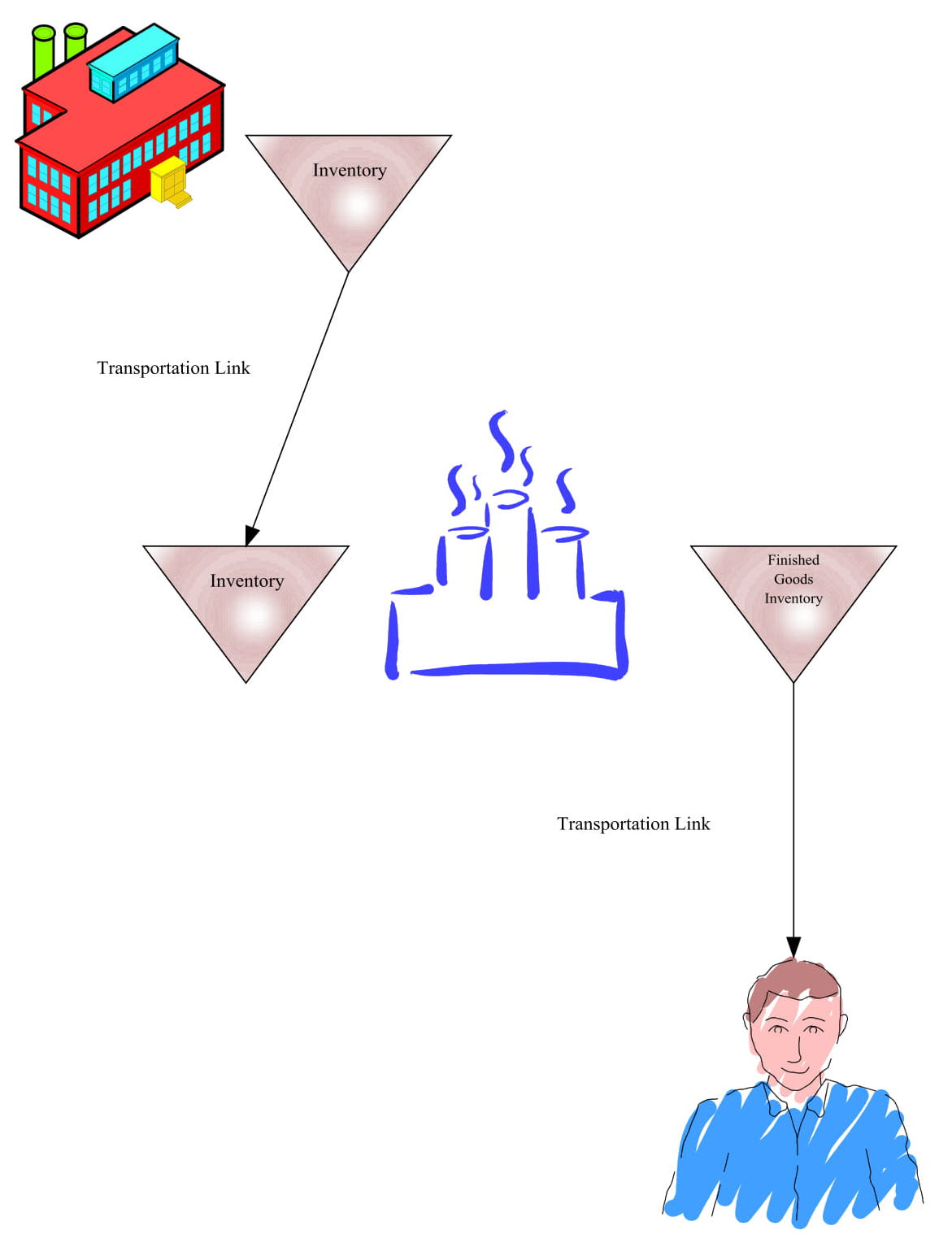
Expected customer demand can vary by month or season of the year. At some times, demand may be far less than production capacity and at some time more. Thus, creating inventory to buffer against demand seasonality is necessary. One approach to doing this is illustrated in this case study.

The effect of the operations of one facility on the decisions made by another facility must be modeled. In this study, equations are used to compute production levels at precedessor plants in a supply chain based on inventory levels at the successor plant, customer demands, and the amount of product in route between the two plants.

The model of a complex system can be implemented using multiple processes. The processes share resources and variables to interact with each other. In this application, nine processes are used to model the supply chain. Variables and resources modeling inventory levels at plant and in route between plants as well as rail fleets are shared between them.

Decisions made within a model may be a function of time. In this application, inventory may be produced in the months prior to peak demand and used only at the time of peak demand.

Supply chain performance is best measured by the service level provide to the customers of retail products. The occasional lack of intermediate inventory for production is acceptable if the customer service level is still satisfactory.

Initial conditions in a supply chain model must include shipments between facilities. In this case, trains are scheduled to arrive at each of the production facilities each day before the expected arrival time of the first train generated by the simulation experiment as a part of the initial conditions.