
15.3: The Case Study
- Page ID
- 31023

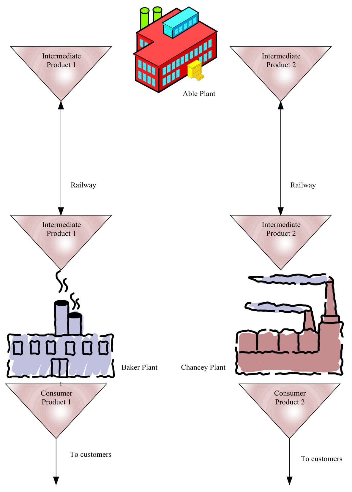
A company owns three plants. Two of the plants, Baker and Chauncey, produce retail products for delivery to customers. A third plant, Able, produces two intermediate products for delivery to the Baker and Chauncey plants. This supply chain is pictured in Figure 15-2.
Product is shipped from the Able plant by rail. There is a separate rail fleet for Able to Baker shipments and for Able to Chauncey shipments.
Customer demand for the retail product made by the Baker plant is triangularly distributed with a minimum of 15 rail cars, a mode of 20 rail cars, and a maximum of 40 rail cars per day. Thus, the average daily demand is 25 rail cars.
Customer demand for the retail product made by the Chauncey plant is seasonal. The average daily demand varies by month of the year as shown in Table 15-1. This data is valid for the next year.
Figure 15-2: Application Study Supply Chain
| Month | Average Daily Demand (Rail Cars) |
| January | 17 |
| February | 18 |
| March | 18 |
| April | 22 |
| May | 23 |
| June | 24 |
| July | 22 |
| August | 21 |
| September | 21 |
| October | 18 |
|
November |
18 |
| December | 18 |
The average of the average daily demands is 20 rail cars. The minimum demand is 70% of the average and the maximum is 130% of the average.
Daily customer demand can include a fractional number of rail cars. However, only full rail cars are shipped with the fractional demand carried over until the next day.
Production capacity at the Able plant is not an issue as sufficient quantities of each intermediate product can be made each day. Production capacity at the Baker and Chauncey plants is constrained. The Baker plant can produce only 35 rail cars per day. The Chauncey plant can produce 27 cars per day.
Production levels are determined daily. Production at the Baker and Chauncey plants can be viewed as occurring in batches equal to one rail car. A rail car of intermediate product sent from the Able plant is required before a batch can be produced. Production of a batch can be modeled as taking 24 hours / daily plant capacity.
Each day at 4:00 A.M. rail cars leave Able plant for the other two plants. There is one train to each plant. All rail cars sent to a plant travel on the same train. Arriving cars at Baker and Chauncey plants are moved into the plant railyard at 12:00 P.M for use the next day. Empty cars leave these plants for return to Able plant at 4:00 A.M. Travel time between Able plant and Baker plant is triangularly distributed with a mean of 7 days, a minimum of 3 days and a maximum of 10 days. Travel time between Able plant and Chauncey plant is triangulary distributed with a mode of 10 days, a minimum of 7 days and a maximum of 20 days. Rail car maintenance will not be modeled.
Rather than construct inventory facilities at the Baker and Chauncey plants, intermediate product remains in rail cars until needed. One rail car at a time is unloaded in preparation for the start of the next batch. Retail product is loaded directly into rail cars for shipment to customers.
15.3.1 Define the Issues and Solution Objective
The objective of the simulation study is to establish values for the operating parameters of the supply chain for the next year, January through December. These include:
- The number of cars in each rail fleet: Able plant to Baker plant as well as Able plant to Chauncey plant.
- The capacity of each inventory: Each of the two intermediate products at Able plant as well as the intermediate and retail product inventories at Baker and Chauncey plants.
- The target retail inventories at Baker and Chauncey plants.
The primary measure of performance is the service level to customers at Baker and Chauncey plants, defined as the number of days when customer demand was met from existing inventory.
15.3.2 Build Models
The first step in analyzing the supply chain is to set initial target retail inventory levels. One way to do this is as follows, remembering that the simulation experiments can be used to find better values for the target inventory level if necessary.
Consider the target retail inventory level at Baker plant. Suppose there was no variation in customer demand or transportation times. The target inventory level would be equal to one day's demand. Product to meet customer demand would be removed from the retail inventory. The day's production would be used to replenish the inventory to meet the next day's demand.
Because of variation, additional inventory is needed to meet customer demands to a specified service level. Suppose a 95% service level is desired. Then the target inventory can be set such that the probability that customer demand is less than the target is 95%. For Baker plant this is 35 rail cars.
For Chauncey plant, the target will vary by month as shown in Table 15-2. Note that the target inventory levels are at or above plant capacity in 4 of 12 months. This may reduce customer service levels below 95%.
| Month | Target Inventory Level (Rail Cars) |
| January | 21 |
| February | 22 |
| March | 22 |
| April | 27 |
| May | 28 |
| June | 29 |
| July | 27 |
| August | 26 |
| September | 26 |
| October | 22 |
| November | 22 |
| December | 22 |
In addition, the average customer demand at Chauncey plant exceeds the plant capacity in May and June. Thus, management has decided to increase daily production by one rail car per day in January, February, and March to prepare for May and June demand. This inventory will be set aside for use starting in April.
It seems prudent to set each of the intermediate product target inventory levels to the same value as the corresponding retail level, at least initially.
Production levels at all three plants are set using the following relationship:
\begin{align}\text{Production = Target Inventory - (Current Inventory + Amount in production)}\tag{15-1}\end{align}
In other words, enough units of a product are sent into production so that the sum of these units, the current inventory and the number of units still in production from previous days is equal to the target inventory.
Capacity constraints are applied at Baker and Chauncey plants. In the number of units sent into production is greater than the daily capacity, some of the units will be produced on subsequent days.
The extra production amount is added at the Chauncey plant as well to help meet customer demand in the months where the target inventory is greater than or equal to the plant capacity. This implies the need for additional intermediate inventory that must be shipped from Able plant.
Shipping volumes are set using the following relationship:
\begin{align}\text{Shipping = (Target Inventory - Current Inventory) (Expected customer demand in expected transportation time Amount in route}\tag{15-2}\end{align}
In addition, the extra production amount is added for shipping between Able and Chauncey plants.
The model consists of nine processes as defined in Table 15-3
| Process Name | Description |
| Able | Daily operation decisions at Able Plant |
| Baker | Daily operation decisions at Baker Plant, including customer service |
| Chauncey | Daily operation decisions at Chauncey Plant, including customer service |
| BakerMake | Production at Baker Plant |
| ChaunceyMake | Production at Chauncey Plant |
| Move2Baker | Train shipment from Able Plant to Baker Plant |
| Move2Chauncey | Train shipment from Able Plant to Chauncey Plant |
| Move2AbleBaker | Train shipment from Baker Plant to Able Plant |
| Move2AbleChauncey | Train shipment from Chauncey Plant to Able Plant |
Important variables in the model are shown in Table 15-4.
| Variable Name | Description |
| Avg2* | Average transporation time from Able plant to * plant (days) |
| AvgRetail* | Average daily customer demand |
| Capacity* | Plant capacity |
| Cars2Cust* | Number of rail cars demanded by customers currently |
| Cars2* | Number of rail cars to be shipped from Able plant currently |
| InRoute* | Number of rail cars currently in route from Able plant |
| ProductionAdd | Number of additional rail cars of retail product to produce daily at Chauncey plant to meet peak demand. The amount varies by month. |
| TargetInvRetail* | Target retail (customer) inventory |
| TargetInvInt* | Target intermediate inventory |
| TargetInvIntAble* | Target intermediate inventory at Able plant |
| *toAble | Number of rail cars currently in route to Able plant |
* = a plant name (Baker, Chauncey)
The Able process is given in the following pseudo-code. This process models the initiation of the shipment of railcars to Baker plant and Chauncey plant as well as the production of intermediate product at Able plant. Entities in this process represent trains and have one attribute:
CarsinTrain: The number of cars in a train
The two intermediate product inventories, one for Baker plant (IntInvAbleBaker) and the other for Chauncey plant (IntInvAbleChauncey), are modeled as resources. The units of each resource correspond to rail cars. The initial number of units of each inventory resource is equal to the target value for that inventory. The same strategy is used to model the retail inventories at Baker (RetailInvBaker) and Chauncey (RetailInvChauncey) plants.
The two rail fleets are modeled as variables: FleetBaker and FleetChaucey. The model is allowed to create as many rail cars in each fleet as needed. Thus, an estimate of the size of each fleet is obtained. The initial size of each rail fleet is zero.
First consider the shipment of rail cars to Baker plant. The number of cars that need to be shipped is incremented using equation 15-2. Suppose the inventory of intermediate product for Baker plant has at least as many cars as the number that need to be shipped. Then all cars that need to be shipped are shipped, the number remaining to be shipped is zero, and the inventory is reduced by the number of cars shipped.
Suppose more cars need to be shipped than are in inventory. Then the train consists of the cars that are in that are inventory. The number remaining to be shipped is reduce by the number in inventory and the number in inventory is set to zero.
In either case, a clone (copy) of the train entity is sent to process Move2Baker.
The modeling logic for a shipment to the Chauncey plant is identical except for the consequences of the expected customer demand varying month to month. All target inventory values for the intermediate product also vary by month.
| Define Arrivals: \(\ \quad \quad\)Time of first arrival: \(\ \quad \quad\)Time between arrivals: \(\ \quad \quad\)Number of arrivals: |
0 1 day Infinite |
| Define Attributes \(\ \quad \quad\)CarsinTrain |
// Rail cars in a train |
| Define Variables \(\ \quad \quad\)AddInv \(\ \quad \quad\)Avg2Baker \(\ \quad \quad\)AvgRetailBaker \(\ \quad \quad\)Cars2Baker \(\ \quad \quad\)Cars2CustBaker \(\ \quad \quad\)InRouteBaker \(\ \quad \quad\)TargetIntInvAbleBaker \(\ \quad \quad\)TargetIntInvBaker \(\ \quad \quad\)Avg2Chauncey \(\ \quad \quad\)AvgRetailChauncey \(\ \quad \quad\)Cars2Chauncey \(\ \quad \quad\)Cars2CustChauncey \(\ \quad \quad\)InRouteChauncey \(\ \quad \quad\)TargetIntInvAbleChaunceyBaker \(\ \quad \quad\)TargetIntInvChauncey |
// Number of additional rail cars needed // Average number of transit days to Baker // Average daily customer demand at Baker // Current number of rail cars to ship from Able to Baker // Current demand in rail cars at Baker // Current number of rail cars in route between Able and Baker // Target intermediate inventory at Able for Baker // Target intermediate inventory at Baker //Average number of transit days to Chauncey //Average daily customer demand at Chauncey //Current number of rail cars to ship from Able to Chauncey //Current demand in rail cars at Chauncey //Current number of rail cars in route -- Able and Chauncey // Target intermediate inventory at Able for Chauncey // Target intermediate inventory at Chauncey |
| Define Resouces \(\ \quad \quad\)FleetBaker \(\ \quad \quad\)FleetChauncey \(\ \quad \quad\)IntInvBaker \(\ \quad \quad\)IntInvChauncey \(\ \quad \quad\)IntInvAbleBaker \(\ \quad \quad\)IntInvAbleChauncey \(\ \quad \quad\)ProductionChauncey \(\ \quad \quad\)RetailInvChauncey \(\ \quad \quad\)SavedInvChauncey |
// Number of rail cars in the Able to Baker fleet // Number of rail cars in the Able to Chauncey fleet // Number of rail cars in intermediate inventory at Baker // Number of rail cars in intermediate inventory at Chauncey // Number of rail cars in intermediate inventory at Able for Baker // Number of rail cars intermediate inventory Able for Chauncey // Production facility at Chauncey // Number of rail cars in finished goods inventory at Chauncey // Number of rail cars in build ahead inventory at Chauncey |
| Process AblePlant Begin \(\ \quad \quad\)Cars2Baker += TargetInvIntBaker - #IntInvBaker/IDLE + (Avg2Baker*AvgRetailBaker-InRouteBaker) \(\ \quad \quad\)If Cars2Baker <= #IntInvAbleBaker/IDLE then \(\ \quad \quad\)Begin \(\ \quad \quad\quad\quad\)CarsinTrain = Cars2Baker \(\ \quad \quad\quad\quad\)Reduce #IntInvBaker/IDLE by CarsinTrain \(\ \quad \quad\quad\quad\)Cars2Baker = 0 \(\ \quad \quad\)End \(\ \quad \quad\)Else \(\ \quad \quad\)Begin \(\ \quad \quad\quad\quad\)CarsinTrain = #IntInvBaker/IDLE \(\ \quad \quad\quad\quad\)Reduce #IntInvBaker/IDLE by CarsinTrain \(\ \quad \quad\quad\quad\)Cars2Baker -= CarsinTrain \(\ \quad \quad\)End \(\ \quad \quad\)Clone to Move2Baker \(\ \quad \quad\)Cars2Chauncey += TargetInvIntChauncey - #IntInvChauncey/IDLE + (Avg2Chauncey*AvgRetailChauncey-InRouteChauncey) \(\ \quad \quad\)If Cars2Chauncey <= #IntInvAbleChauncey/IDLE then \(\ \quad \quad\)Begin \(\ \quad \quad\quad\quad\)CarsinTrain = Cars2Chauncey \(\ \quad \quad\quad\quad\)Reduce #IntInvChauncey/IDLE by CarsinTrain \(\ \quad \quad\quad\quad\)Cars2Chauncey = 0 \(\ \quad \quad\)End \(\ \quad \quad\)Else \(\ \quad \quad\)Begin \(\ \quad \quad\quad\quad\)CarsinTrain = #IntInvChauncey/IDLE \(\ \quad \quad\quad\quad\)Reduce #IntInvChauncey/IDLE by CarsinTrain \(\ \quad \quad\quad\quad\)Cars2Chauncey -= CarsinTrain \(\ \quad \quad\)End \(\ \quad \quad\)Clone to Move2Chauncey \(\ \quad \quad\)Wait until Midnight \(\ \quad \quad\)AddInv = TargetIntInvBaker - #IntInvAbleBaker/Idle \(\ \quad \quad\)If (#FleetBaker/IDLE < AddInv) Then increase #FleetBaker/IDLE by (AddInv - #FleetBaker/IDLE) \(\ \quad \quad\)Make FleetBaker/AddInv BUSY \(\ \quad \quad\)Reduce #IntInvAbleBaker/IDLE by AddInv \(\ \quad \quad\)AddInv = TargetIntInvChauncey(Month) - #IntInvAbleChauncey/Idle If (#FleetChauncey/IDLE < AddInv) Then increase #FleetChauncey/IDLE by (AddInv - #FleetChauncey/IDLE) \(\ \quad \quad\)Make FleetChauncey/AddInv BUSY \(\ \quad \quad\)Reduce #IntInvAbleChauncey/IDLE by AddInv End |
|
After the train shipments are initiated, time is delayed until midnight when the inventories are updated. Since there is no constraint on production at Able plant, each inventory is simply reset to the target value. In addition, each unit in inventory is stored in a rail car. If there are insufficient idle rail cars at Able plant, additional units of each fleet resource are created.
The remaining discussion of the model will focus on the Chauncey plant. Baker plant operates in an identical way except that time varying average demand is not a factor.
The process Move2Chauncey is shown in the following pseudo-code. The number of rail cars in route to Chauncey is incremented by the number of cars in the train, CarsinTrain. The time delay for movement from Able to Chauncey is determined as a sample from the triangular distribution with minimum 7, mode 10, and maximum 20 days. All trains arrive at midnight. The number of cars in the intermediate product inventory at the Chauncey plant is recorded by increasing the number of idle units of the resource IntInvChauncey. The arriving cars are subtracted from the number of cars in route to the Chauncey plant.
Process Move2Chauncey
Begin
\(\ \quad \quad\)InRouteChauncey +- CarsinTrain
\(\ \quad \quad\)Wait for Triangualar 7, 10, 20 days \(\ \quad \quad\)//Train from Able to Chauncey
\(\ \quad \quad\)Wait until Midnight
\(\ \quad \quad\)Increase #InvIntChauncey by CarsinTrain
\(\ \quad \quad\)InRouteChauncey -= CarsinTrain
End
Next consider the daily operations at the Chauncey plant. This involves determining the number of rail cars of product demanded by customers, the number of cars that can be shipped from inventory to meet this demand and the number of rail cars of the retail product to produce to replenish the inventory. Additional cars of retail product may need to be produced and saved to meet peak demand. Such cars already in inventory may or may not be available to meet current demand.
The process begins by adding the customer demand for the current day to the currently unfilled customer demand (the variable Cars2Cust). The demand is a sample from a triangular distribution whose mode depends on the month of the year, whose minimum is 70% of the mode and whose maximum is 130% of the mode and can result in a fractional number of rail cars. Only whole rail car loads are shipped so fractional demand, as well as unmet demand, is carried forward to the next day.
If the number of rail cars in the regular inventory is sufficient to meet the customer demand, then the inventory is reduced by the number of rail cars demanded and the remaining customer demand is reduced by the same quantity. If the demand is greater than the number of rail cars in regular inventory, the entire inventory is used to partially meet the demand. The inventory and demand variables are updated accordingly. If the month is April through December, the saved inventory can used to meet the remaining demand, partially or completely.
Service level observations are recorded. If all demand is met, the service level for the day is 100. Otherwise, the service level is zero.
The regular inventory is replenished to the target level by creating an order to produce more rail cars of retail product. The number of rail cars to produce is given by equation 15-1. The number of rail car loads in production is incremented by the right hand side of the same equation.
The saved inventory is built up each day by the number cars depends on the month of the year and is specified in the variable ProductionAdd(Month). Thus, an order for ProductionAdd(Month) additional rail cars is created.
Each order entity corresponds to a single rail car's volume of production and has one attribute.
IsSaved: Whether or not the rail car is a part of the saved inventory (1 Yes; 0 No or regular inventory.)
The Chauncey plant process is given in the following pseudo-code.
| Define Attributes IsSaved |
// Is rail car part of saved inventory |
| Define Variables WholeCars OrderSize |
// Integer portion of demand in rail cars // How much to produce in rail cars |
|
Process ChaunceyPlant |
|
Chauncey plant production is modeled by process MakeChauncey, which is shown in the following pseudocode. Each entity represents an order to produce one rail car. The entity waits for one rail car sized unit of the intermediate product inventory. After the intermediate inventory is obtained, the entity waits for its turn in the Chauncey production facility. The production time is 1440 minutes (in a day) / 27 ( the daily production capacity). Thus, the number of units made per day is limited to the capacity. The newly made unit is added to the appropriate inventory (regular or saved). The rail car containing the intermediate product is sent to wait for the next train to Able plant by adding one to the count of the number of rail cars on the train.
Process MakeChauncey
Begin
\(\ \quad \quad\)Wait until IntInvChauncey/1 to be IDLE
\(\ \quad \quad\)Make IntInvChauncey/1 Busy
\(\ \quad \quad\)Wait until ProductionChauncey/1 is IDLE
\(\ \quad \quad\)Make ProductionChauncey/1 Busy
\(\ \quad \quad\)Wait for 1440/27 minutes
\(\ \quad \quad\)Make ProductionChauncey/1 IDLE
\(\ \quad \quad\)Reduce #IntInvChauncey/Busy by 1
\(\ \quad \quad\)If IsSavedInv = 0 then
\(\ \quad \quad\)Begin
\(\ \quad \quad\quad \quad\)Increase #RetailInvChauncey/IDLE by 1
\(\ \quad \quad\quad \quad\)RetailProdChauncey -=1
\(\ \quad \quad\)End
\(\ \quad \quad\)Else Increase #SavedInvChauncey/IDLE by 1
\(\ \quad \quad\)Chauncey2Able +=1
End
The movement of empty cars from Chauncey plant to Able plant is modeled by process MoveChauncey2Able as shown in the following pseudocode. The number of cars in the train is the number cars containing intermediate inventory that was consumed since the last train departed. The trip is made and the train arrives at midnight to Able plant. One unit of the FleetChauncey resource is freed for each car in the train.
Define Arrivals:
\(\ \quad \quad\)Time of first arrival: 0
\(\ \quad \quad\)Time between arrivals: 1 day
\(\ \quad \quad\)Number of arrivals: Infinite
Process Move2AbleChauncey
Begin
\(\ \quad \quad\)CarsinTrain = Chauncey2Able
\(\ \quad \quad\)Chauncey2Able = 0
\(\ \quad \quad\)Wait for 7, 10, 20 days
\(\ \quad \quad\)Wait until Midnight
\(\ \quad \quad\)Make FleetChauncey/CarsinTrain IDLE
End
It is important to note when and how each process is initiated. An entity is sent to each of the plant processes: Able, Baker, and Chauncey once each day at midnight. An entity is sent to each process that moves trains to Able plant: Move2AbleBaker and Move2AbleChauncey at the time of daily train departure, 4 A.M. The MakeBaker and MakeChauncey processes are initiated by the Baker and Chauncey plant processes respectively after the number units to make to replenish the inventory has been determined. The Move2Baker and Move2Chauncey processes are initiated by the Able plant process after the number of rail cars to ship to each has been determined.
15.3.3 Identify Root Causes and Assess Initial Alternatives
The design of the initial simulation experiment is shown in Table 15-5. Since the customer demand data is valid for one year, a terminating experiment of length one year is used.
Model parameters are the inventory target levels. Establishing inventory target levels is a primary objective of the simulation study. This will done by setting the target levels in the manor previously described and detemining the resulting system performance. The performance in measured by the customer service level at Baker and Chauncey plants as well as the size of each fleet. In addition, the waiting time of orders for intermediate product at Baker and Chauncey plants so production can begin will be measured. Excessive waiting time could lower customer service levels. Only the waiting time for orders that had to wait is recorded.
There are four random streams, two for transportation times to and from Able plant and two for customer demand at Baker and Chauncey plants. Twenty replicates will be made.
Ideally, the level of each inventory at the end of each day should be the target value. Thus, the target value is used for the initial inventory level.
Trains arrive to Baker and Chauncey plant daily on the average. However, the first shipments from Able plant will not arrive to Baker and Chauncey plants until day 7 and 10 on the average. Thus, shipments must be scheduled to arrive to Baker and Chauncey plants on the preceding days as part of the initial conditions. Shipment size is the average number of rail cars arriving to the plant per day. This is equal to the average customer demand at that plant.
| Element of the Experiment | Values for This Experiment |
| Type of Experiment | Terminating |
| Model Parameters and Their Values | 1. Retail inventory target levels set to the 95% point of the customer demand distribution 2. Intermediate inventory target levels at Baker and Chauncey plants initially set to the same value as corresponding retail inventory target level 3. Intermediate inventory target levels at Able plant initially set to the same value as the corresponding inventory at Baker or Chauncey plant |
| Performance Measures | 1. Service level to customers at Baker plant 2. Service level to customers at Chauncey plant 3. Fleet size: Able to Baker 4. Fleet size: Able to Chauncey 5. Order waiting time for intermediate inventory at Baker plant 6. Order waiting time for intermediate inventory at Chauncey plant |
| Random Number Streams | 1. Transportation time between Able plant and Baker plant 2. Transportation time between Able plant and Chauncey plant 3. Customer demand at Baker plant 4. Customer demand at Chauncey plant |
| Initial Conditions | 1. All inventory levels set equal to their target 2. Intermediate inventory arrivals to Baker and Chauncey plants as discussed in the text |
| Number of Replicates | 20 |
| Simulated End Time | 1 year |
Simulation results are shown in Table 15-6.
| Fleet Size (Rail Cars) | Service Level | Wait for Inventory (Hours) | ||||
| Replicate | Baker | Chauncey | Baker | Chauncey | Baker | Chauncey |
| 1 | 501 | 666 | 43 | 5 | 31 | 33 |
| 2 | 500 | 722 | 55 | 18 | 29 | 35 |
| 3 | 502 | 671 | 49 | 7 | 30 | 36 |
| 4 | 468 | 724 | 68 | 26 | 30 | 33 |
| 5 | 467 | 700 | 85 | 72 | 26 | 35 |
| 6 | 501 | 704 | 61 | 33 | 29 | 31 |
| 7 | 500 | 684 | 48 | 9 | 34 | 36 |
| 8 | 502 | 719 | 54 | 44 | 31 | 34 |
| 9 | 494 | 724 | 39 | 6 | 32 | 33 |
| 10 | 495 | 698 | 43 | 21 | 30 | 35 |
| 11 | 486 | 732 | 61 | 39 | 28 | 33 |
| 12 | 484 | 709 | 60 | 28 | 28 | 32 |
| 13 | 481 | 749 | 64 | 7 | 29 | 32 |
| 14 | 489 | 675 | 68 | 51 | 28 | 32 |
| 15 | 534 | 717 | 61 | 39 | 31 | 32 |
| 16 | 472 | 722 | 288 | 24 | 33 | 34 |
| 17 | 501 | 737 | 54 | 9 | 32 | 37 |
| 18 | 489 | 717 | 44 | 38 | 33 | 32 |
| 19 | 488 | 736 | 52 | 26 | 30 | 33 |
| 20 | 476 | 695 | 51 | 18 | 32 | 33 |
| Average | 492 | 710 | 54 | 26 | 30 | 33 |
| Std. Dev. | 15 | 23 | 13 | 18 | 2 | 2 |
| 99% CI Lower Bound | 482 | 695 | 46 | 15 | 29 | 32 |
| 99% CI Upper Bound | 501 | 725 | 62 | 37 | 32 | 34 |
Service level values are unexceptably low. Order waiting time for intermediate inventory averages greater than one day at each plant. An average of 1339 orders per replicate waited for intermediate inventory at the Baker plant with an approximate 99% CI of (1152, 1526) while an average of 1094 orders per replicate waited for intermediate inventory at the Chauncey plant with an approximiate 99% CI of (949, 1238).
These results lead to a second alternative. The target intermediate inventory at Baker plant is increased by the expected customer demand in one day as the waiting time for intermediate inventory averages about 1.25 days. Similarly, the target inventory at Chauncey plant is increased by the expected customer demand in two days as the waiting time for intermediate inventory is about 1.4 days. Otherwise the simulation experiment is the same as shown in Table 15-5. Results are shown in Table 15-7.
| Fleet Size (Rail Cars) | Service Level | Wait for Inventory (Hours) | ||||
| Replicate | Baker | Chauncey | Baker | Chauncey | Baker | Chauncey |
| 1 | 520 | 770 | 93 | 97 | 24 | 30 |
| 2 | 483 | 795 | 97 | 96 | 24 | 47 |
| 3 | 501 | 771 | 93 | 90 | 24 | 33 |
| 4 | 492 | 763 | 93 | 99 | 24 | 26 |
| 5 | 516 | 778 | 91 | 94 | 25 | 27 |
| 6 | 499 | 744 | 93 | 95 | 30 | 25 |
| 7 | 502 | 750 | 95 | 97 | 24 | 26 |
| 8 | 532 | 819 | 91 | 91 | 25 | 30 |
| 10 | 494 | 846 | 96 | 97 | 25 | 39 |
| 11 | 516 | 782 | 90 | 93 | 25 | 29 |
| 12 | 504 | 784 | 95 | 97 | 24 | 28 |
| 13 | 497 | 813 | 94 | 96 | 29 | 34 |
| 14 | 499 | 774 | 92 | 99 | 27 | 36 |
| 15 | 505 | 799 | 97 | 93 | 26 | 28 |
| 16 | 487 | 773 | 95 | 96 | 24 | 41 |
| 17 | 492 | 748 | 96 | 96 | 28 | 32 |
| 18 | 524 | 808 | 93 | 96 | 25 | 33 |
| 19 | 511 | 808 | 94 | 95 | 25 | 25 |
| 20 | 502 | 779 | 93 | 95 | 25 | 32 |
| Average | 504 | 785 | 94 | 96 | 25 | 32 |
| Std. Dev. | 13 | 26 | 2 | 3 | 2 | 7 |
| 99% CI Lower Bound | 496 | 769 | 92 | 94 | 24 | 28 |
| 99% CI Upper Bound | 512 | 802 | 95 | 97 | 26 | 37 |
Results show that the approximate 99% confidence intervals for the service level at both the Baker plant and the Chauncey plant contain the target service level of 95%. The fleet size required for the Chauncey plant is 785 cars and the fleet size required for Baker plant is 504 cars. An average of 122 orders per replicate waited for intermediate inventory at the Baker plant with an approximate 99% confidence interval of (83, 161) while an average of 124 orders per replicate waited for intermediate inventory at the Chauncey plant with an approximate 95% confidence interval of (100, 148). Note that number of orders waiting at each plant has dropped by about an order of magnitude.
Since service levels are acceptable for this alternative, inventory capacity can be examined. The retail inventories at Baker and Chauncey plant can by design not exceed the target. The same is true for the intermediate inventories at Able plant. Thus, only the inventory capacities to be set are the intermediate inventories at Baker and Chauncey plant. The approximate 99% confidence interval for the maximum number of rail cars in the intermediate inventory at Baker plant is (135, 145) with an average of 140. The approximate 99% confidence interval for the same quantity at Chauncey plant is (155, 170) with an average of 162.
15.3.4 Review and Extend Previous Work
Management was willing to except a slightly less than 95% service level at Baker plant. Fleet sizes of 504 for Able to Baker and 785 for Able to Chauncey will be used. The number of orders waiting for intermediate inventory as well as the average waiting time were felt to be acceptable.
The target inventory levels are as follows. Note that target inventory values associated with Chauncey plant vary by month.
| Retail inventories: | 35 at Baker plant, the 95% point of the demand distribution as shown in Table 15-2 at Chauncey plant. |
| Intermediate inventories: | 60 (35 + 25 = the expected demand in one day) at Baker plant and for the Baker plant intermediate inventory at Able plant 35 + 2 * the monthly value shown in Table 15-1 for the Chauncey plant |
| Inventory capacities were set as follows. | |
| Customer inventories: | Same as target inventories. |
| Intermediate inventories: | Able plant - Same as target inventories. Baker plant - Same as the average maximum of 140 rail cars Chauncey plant - Same as the average maximum of 162 rail cars |
15.3.5 Implement the Selected Solution and Evaluate
The supply chain will be operated with the above parameters. Service level performance will be monitored.