16.3: The Case Study

The following case study is a subset of one described by Warber and Standridge (2002). A package sorting hub is entering an expansion phase. The number of unloading banks, primary sorters and secondary sorters is increasing to support processing an increased volume of packages. Secondary sorter operations are of particular interest.

16.3.1 Define the Issues and Solution Objective

The level of staffing is a significant cost component for a transfer hub. Thus, the number of workers assigned to loading out bound trucks is at issue. Management believes that a worker can support more than one secondary sorter lane at a time. For example, a worker supporting two lanes would wait until a package arrives to one of the two lanes, walk to that lane, place the package on the truck, and return to look for the next arriving package on either lane. Note that in addition to the time to load a package into a truck, the walking time to a lane must be taken into account.

The number of workers to assign to the secondary sorter must be determined. The number of workers should be minimized to reduce costs. At the same time, loading delays are detrimental to hub operations. Thus, the time to load a package should be minimized. These two operating criteria are in conflict and a suitable balance between the two must be found.

A simulation study will be done to determine the number of workers to assign per secondary sorter. Trucks containing packages arrive to the terminal between 4:00 P.M. and 8:00 P.M. each day. It is estimated that on the average 8000 of these packages will be processed by the secondary sorter of interest. Since many packages are also sent to other secondary sorters, the time between arrivals the secondary sorter of interest is considered to be an exponentially distributed random variable with mean 4 hours / 8000 packages or 1.8 seconds.

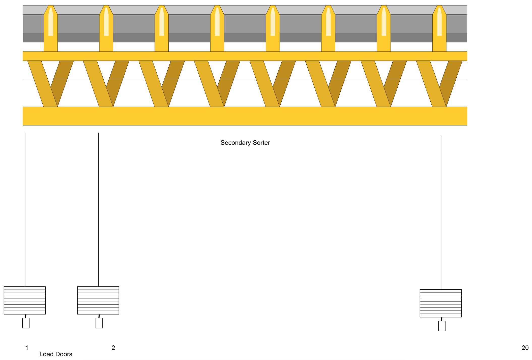
The secondary sorter serves 20 loading lanes each leading to a loading dock. A package is equally likely to be routed to any of the loading lanes. The distance between loading lanes is 10 feet measured from the center point of one loading lane to the center point of the next. A detailed drawing of the secondary sorter of interest is given in Figure 16-2.

The distance from the secondary sorter to a loading door is 37 feet. The total length of the secondary sorter conveyor is 250 feet. Conveyor speed is 1 foot per second.

Loading time consists of two components: the time for a worker to remove a package from the end of the loading lane and place it properly in the a truck and the time for the worker to walk to a loading lane. The former can be modeled as a random variable since the location of a particular package in a truck depends on the packages currently in the truck. Experience has found the loading time to be highly variable with a mean of 8 seconds. Thus, loading time is considered to be exponentially distributed.

The time for a worker to walk to a loading lane depends on how many lanes the worker serves. If the worker serves two lanes and waits half way between them for an arriving package, the walking distance is five feet. Assuming the average walking speed is 2 miles per hour, the average walking time is about 1.7 seconds. This time is about 21% of the average time to place a package on a truck and thus is a significant factor in determining system performance.

Figure 16-2: Secondary Sorter and Load Area

16.3.2 Build Models

The model of the secondary sorter operations must take into account the following system components.

1. Arrival of packages to the secondary sorter between 4 P.M. and 8 P.M. with an exponentially distributed time between arrivals with a mean of 8 seconds.
2. Package movement along the secondary sorter conveyor until the lane corresponding to the loading door is reached.
3. Package movement to the end of the lane.
4. Loading of the package on the truck.
5. Worker assignment to lanes including walking time to a lane.

Arriving entities model packages and have the following attributes.

1. Lane: Loading lane assignment, 1, 2, ..., 20.
2. TimeArriveLane: Time of arrival to the end of a lane.
3. LaneWorker: ID of the particular worker resource assigned to lane Lane.

The latter attribute allows the time a package waited for a worker for loading to be collected.

Model logic is shown in the following pseudocode. Packages arrive according to an exponential distribution with mean 1.8 seconds. The lane from which the package will be loaded is computed as a sample from a uniform distribution between 1 and 21. Thus, each of the lanes 1 through 20 is equally likely. The package moves on the secondary sorter conveyor at the rate of 1 foot per second to the selected lane. Then the package moves down the lane to its end at the same rate. The arrival time at the end of the lane is noted. The package waits at the end of the lane for the worker serving that lane. The waiting time is collected. The worker walks to the lane in 1.7 seconds and then loads the package in an exponentially distributed time with a mean of 8 seconds. After this task, the worker becomes IDLE again.

---

Define Arrivals Time of first arrival: Time between arrivals: Number of arrivals:	0 Exponential 1.8 seconds Infinite
Define Attributes Lane TimeArriveLane LaneWorker	// Loading lane assignment, 1, 2, ..., 20. // Time of arrival to the end of a lane. // ID of the particular worker resource assigned to lane Lane.
Define Resources Worker(2)	// Lane workers
Process SecondarySorter Begin Lane = Integer (Uniform 1, 21) Wait for (1 sec * distance to lane in feet) Wait for (1 sec * length of lane conveyor in feet) TimeArriveLane = Clock LaneWorker = (Lane+1)/2 Wait until Worker(LaneWorker)/1 is IDLE Make Worker(LaneWorker)/1 BUSY Tabulate (Clock-LaneArrivalTime) in WaitforWorker Wait for 1.7 seconds Wait for Exponential 8 seconds Make Worker(LaneWorker)/1 IDLE End	// Select Lane // Move to lane // Move to load area // Select lane worker // Worker walks to lane // Worker loads truck

---

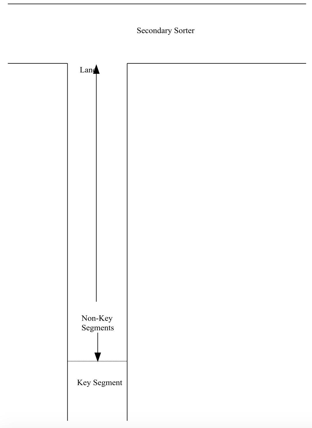
Model logic for a conveyor deserves more detailed discussion. Consider a lane conveyor. The conveyor is divided into segments. Each segment can contain one package so each segment is the size of a package. The segment at the end of the lane is called a key segment. The key segment is modeled as a resource so that only one package can occupy the key segment at a time. Packages waiting for the key segment to become idle occupy the segments physically preceding the key segment. If enough packages are waiting, the lane could become full and block the secondary sorter conveyor.

When modeling a conveyor, the size of entities traveling on the conveyor and the key segments must be specified along with the conveyor speed. The use of the non-key segments as queuing space for a key segment must be included in the model. Figure 16-3 summarizes these ideas. An entity moves on the lane until it reaches the non-key segment closest to the key segment that is not occupied by another entity. Each entity waits to enter the key segment. As an entity departs the key segment, all remaining waiting entities move one non-key segment closer to the key segment.

Fortunately, the above logic is included in the modeling constructs of many simulation languages. Thus, the modeler is required only to specify the conveyor parameters, for example package size, conveyor speed, conveyor length, and key segment location.

Figure 16-3: Model of a Lane Conveyor

16.3.3 Identify Root Causes and Assess Initial Alternatives

Management desires that the workers be kept as busy as possible. On the other hand, ergonomic considerations require worker rest and personal time to be about 20% of the work period. Thus, an average worker utilization of 80% is sought and this quantity is one performance measure. The time a package waits for a worker before loading is also of interest.

One model parameter will be varied, the number of lanes server by a worker, either 2 or 3. Note that worker walking time to a lane will increase when 3 lanes are served. The worker will stand at the middle lane of the three being served. The walking distance to the middle lane is therefore neglibile. The walking distance to each of the other two lanes is 10 feet. Thus, the average walking distance increases from 5 feet to 6.67 feet and the average walking time increases from 1.7 seconds to 2.3 seconds. Having each worker serve 3 lanes instead of 2 reduces the number of workers from ten to seven. Six of the seven workers serve 3 lanes and the seventh server the remaining two lanes.

Since trucks arrive with packages between 4 P.M. and 8 P.M. each day, a terminating simulation experiment of duration 4 hours is employed. Twenty replicates will be made. Since there are no packages at the secondary sorter at 4 P.M., the initial conditions are all lanes empty and all workers idle.

There are three random number streams used in the model, one for package arrivals, one for lane assignments, and one for package loading time onto trucks.

The experiment is summarized in Table 16-1.

Table 16-1: Simulation Experiment Design for the Secondary Sorter

Element of the Experiment	Values for This Experiment
Type of Experiment	Terminating
Model Parameters and Their Values	Number of lanes served by one worker (2 or 3)
Performance Measures	1. Average utilization over all workers 2. Waiting time for a worker
Random Number Streams	1. Time between arrivals 2. Lane assignment for a package (1-20) 3. Loading time
Initial Conditions	Empty and idle
Number of Replicates	20
Simulation End Time	4 hours

Simulation results for the cases where a worker serves 2 and 3 lanes are shown in Table 16-2. Average worker utilization is the average utilization of all workers in the first case and of only those workers serving 3 lanes in the second case.

Table 16-2: Average Worker Utilization and Package Waiting Time for a Worker at the Secondary Sorter

	Worker Serves Two Lanes		Worker Serves Three Lanes
Replicate	Average Package Waiting Time (sec)	Average Worker Utilization	Average Package Waiting Time (sec)	Average Worker Utilization
1	3.1	0.533	10.7	0.843
2	2.8	0.520	9.8	0.832
3	2.9	0.529	10.3	0.839
4	2.9	0.535	10.8	0.845
5	2.8	0.529	10.4	0.845
6	2.9	0.528	10.4	0.842
7	2.9	0.527	10.4	0.837
8	3.0	0.527	10.1	0.839
9	3.0	0.535	10.3	0.844
10	3.1	0.538	10.6	0.855
11	3.0	0.530	10.2	0.841
12	2.9	0.527	9.9	0.835
13	3.1	0.533	10.4	0.844
14	3.2	0.546	11.3	0.870
15	2.9	0.537	10.8	0.853
16	2.9	0.530	10.3	0.843
17	2.9	0.536	10.7	0.852
18	3.1	0.536	11.4	0.858
19	2.9	0.534	10.7	0.849
20	3.0	0.526	10.3	0.836
Average	3.0	0.532	10.5	0.845
Std. Dev.	0.096	0.00560	0.398	0.00903
99% CI Lower Bound	2.9	0.528	10.2	0.839
99% CI Upper Bound	3.0	0.535	10.7	0.851

Note that in neither case does the approximate 99% confidence interval contain the target utilization of 80%. Package average waiting time increases by about 3.5 times when a worker serves three lanes instead of 2.

16.3.4 Review and Extend Previous Work

Management was disappointed that neither assigning 2 or 3 lanes to a worker produced the desired utilization of 80%. The slightly higher utilization of 84.5% on the average was deemed unacceptable since upper bound of the 99% confidence interval was 85.1%. A worker utilization of 53.2% was deemed too low and thus too costly.

The following alternative was proposed. Each worker would serve 2 lanes alone plus sharing the responsibility for a third lane with another worker. This would increase the number of workers from seven serving 3 lanes each to eight serving 2.5 lanes each. Thus, the simulation project process was restarted at the Build Models step.

16.4.1 Build Models

The average walking time when a worker serves two lanes and shares responsibility for a third lane was computed as follows. A worker stands in the same position as when serving 2 lanes. Thus, the average walking time is 1.7 seconds for 80% of the package loading operations. For the other 20% of the package loads, the walking distance is 15 feet, which requires 5.1 seconds on the average. Thus, two walking times must be included in the model.

A new version of the model was created to model two workers sharing responsibility for every third lane. The shared lanes are 3, 8, 13, and 18. No changes to model logic are required for non-shared lanes. For shared lanes, the changes to model logic are as follows.

1. Wait for either lane worker to perform the loading operation, whichever one becomes IDLE first.
2. Use the walking time to a shared lane, 5.1 seconds.
3. Free whichever worker performed the loading operation.

16.4.2 Identify Root Causes and Assess Initial Alternatives

The experiment is the same as the one define in Table 16-1 except for the performance measures. Waiting time for each of two types of packages is required: those using lanes served by one worker alone and those using lanes servered by two workers.

Simulation results comparing the two cases are shown in Table 16-3.

In the shared lanes scenario, all workers serve the same number of lanes, 2.5. The average worker utilization is 66.4%, less than the desired 80% target but more than in the case where each worker serves only two lanes. Average package waiting time is about half of that in the workers serve 3 lanes case. Average package waiting time is less on the shared lanes than on the lanes that do not share a worker.

16.4.3 Implement the Selected Solution and Evaluate

Management was disappointed that the target worker utilization of 80% could not be achieved but satisfied with the using eight workers instead of the ten required by the case in which a worker servers two lanes only. Average package waiting time was deemed satisfactory.