17.3: The Case Study1

The case study has to do with confirming the operational effectiveness of the design of a new AGV system as well as determining the number of vehicles needed. Load movement requests can be modeled as having a constant time between arrivals. However, the orgin and destination points are stochastic. That is not all requests for material movement can be predetermined. The discussion and examples of AGV systems in Askin and Standridge (1993) form the basis for this case study.

17.3.1 Define the Issues and Solution Objective

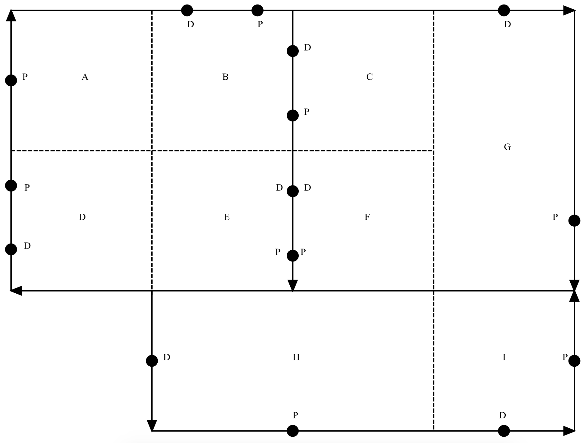
The design of a new AGV system to serve nine workstations as shown in Figure 17-2. Each shorter edge corresponds to 50 feet and each longer edge to 100 feet. AGV's move in one direction only on each bold edge as indicated by the arrows. There is no AGV movement on dashed edges. The letters in the center of a square are the work station ID's. The numbers near the edges are the control segment ID's. Idle AGV's wait where at the dropoff point of their last load.

The pickup and dropoff points for each workstation are indicated using the letters P and D respectively. Note that stations 5 and 6 share these points.

Table 17-1 gives the average number of material moves between workstations per 16 hour day. This information forms the distribution of pickup point to dropoff point AGV movements. Each individual movement can be determined as a random sample from this distribution. The time between material moves is a constant 90 seconds (57600 seconds per day / 640 moves).

A material move requires an AGV to move from it current location to the pickup point and then from the pickup point to the dropoff point. Each AGV moves at the rate of 5 feet per second and takes 30 seconds for each drop-off and each pick-up.

---

¹ Todd Frazee assisted with the development of this case study.

---

Figure 17-2: AGV System Layout

The design shown in Figure 17-2 was developed using analytic methods. The following principles were applied.

1. Vehicles move in only one direction on path.
2. The dropoff point for a station should precede the pickup point with respect to vehicle movement.
3. Dropoff and pickup points should be placed on control segments with low utilization to avoid other vehicles waiting for dropoffs and pickups to be completed.
4. Movement of empty vehicles should be minimized. Thus after a dropoff is completed, the vehicle should wait on the same control segment for a possible pickup on that segment.

Other analytic methods were used to estimate that 2 AGV's would be needed in the system. These analytic methods were used to compute each of the five components of total vehicle utilization time: loaded travel time, travel time while empty, blocked time, load time, and unload time. These computations are based on knowledge of the number of loads to be moved between each pair of workstations (the information shown in Table 17-1) as well as AGV travel speeds and the shortest path between each pair of workstations.

Loaded travel time, load time, and unload time are straightforward to compute. A lower bound on travel time while empty can be computed using an optimization algorithm. Blocked time was assumed to be zero for this system since the number of AGV's need was only 2.

Table 17-1: Average Number of Material Moves between Work Stations

From Work Station	To Work Station	Average Number of Moves
A	B	40
A	C	25
A	D	30
A	E	10
A	F	10
A	G	20
A	H	5
A	I	10
B	C	40
B	E	30
B	G	10
B	H	10
C	G	50
C	I	10
D	B	5
D	C	10
D	F	10
E	D	100
F	D	60
G	F	40
G	I	40
H	D	10
H	F	5
I	E	60
Total		640

Management wishes to confirm the operationally effectiveness of AGV system as designed. The primary performance criteria is time between the request for a load to be moved and the completion of the move. Both the maximum and average time are interest. Assessing the number of AGV's needed is also important since blocked time was ignored and only a lower bound on travel time while empty was obtained. There is concern that 2 AGV's are not sufficient.

17.3.2 Build Models

It is helpful to take a generic perspective to modeling AGV systems. The control segments and control points that comprise the paths taken by the vehicles between workstations can be data input, expressed most often as a graphical drawing. In this case, the graphical drawing used for input this information is the one in Figure 17-2. Other inputs include where vehicles park when they become idle and vehicle speed. Vehicles can be viewed as resources. This generic view is implemented in some simulation environments.

In addition, a process model describing the movement of loads through the AGV system, perhaps including processing at workstations, is needed. A request to move a load is the entity flowing through the process. The following are the major steps in the process model.

1. Arrival of a request for an AGV to move a load from one workstation to another.
2. Waiting for an idle AGV.
3. Selection of the idle AGV nearest to the pickup point for the load.
4. Movement of that AGV from where it is parked to the pickup point.
5. Movement of the same AGV from the pickup point to the dropoff point.

Attributes of the entity are the following:

FromStation	The station where the load is to be picked up.
ToStation	The station where the load is to be dropped off.
ArriveTime	Simulation time that the request for load movement is made.

Analytic algorithms for determining the shortest path from one workstation to another are known and can be implemented within a simulation environment that supports modeling AGV systems. In most cases, the number of feasible paths between any pair of workstation should be few in number. Otherwise, the system would be too complex to operate. For example, consider the number of paths from workstation A in Figure 17-2 to each of the other eight workstations. There is only one path to workstations B, C, E, F, and G. There are two paths to the other workstations: D, H, and I. However, one of the two paths is obviously shorter.

One issue that is unique to modeling AGV systems is contention among the vehicles for the same control segment or control point. All vehicles travel at the same speed so one cannot overtake another as long as both are moving in the same direction. Contention occurs when one vehicle is stopped at a pickup or dropoff point and another vehicle needs to pass through such a point enroute somewhere else. In this case, the second vehicle needs to stop to wait for the first vehicle to leave the pickup or dropoff point.

In addition, contention can occur when two vehicles coming from opposite directions arrive at the same intersection at the same time. One vehicle needs to stop or slow down to let the other vehicle pass. There are two such intersections in the AGV system shown in Figure 17-2. One is at the right side of the boundary between workstations G and I. The other is at the center of the upper boundary of workstation H where the path dividing workstations E and F ends.

One system performance criterion is the time between the request for moving a load and completion of the move. Thus, it may seen desirable to have as many AGV's in the system as possible to minimize this time. This strategy is similar to increasing the number of machines at a workstation to minimize cycle time at the station that was employed in previous chapters. However, increasing the number of AGV's also increases the contention for control points and control segments. Thus, such increases may be counter productive and must be tested using simulation.

The modeling logic described above follows in pseudo English. AGV's are modeled as resources as are pickup and dropoff points. Each AGV has an attribute, CurrentLoc, giving its current location. Resources are also used to model intersections where vehicles can enter from more than one direction.

Travel along a path is comprised of a series of steps as modeled by Process MoveOnPath with parameters FromLoc and ToLoc. Each step represents travel between the current AGV location and the next pickup point, dropoff point, or intersection on the path. Each of these is modeled as resource that must be acquired to traverse that part of the path and freed after such movement is accomplished.

The next pickup point, dropoff point, or intersection and the distance to it are exacted from the data input describing the AGV system that was given as a graphical drawing. In this case, travel time can be modeled as distance traveled * AGV speed. It is possible to include acceleration and deacceleration if desired. When the destination control point is reached, travel ends. Otherwise travel to the next pickup point, dropoff point, or intersection commences.

The process AGV System makes use of the process MoveOnPath. Arrivals to the process are requests for load movement that occur every 90 seconds in this case. Entity attributes are assigned: the workstation where the load currently resides, the workstation to which the load must be transported, and the simulation time the request arrives. The idle AGV closest to the workstation station where the load currently resides is chosen. If there are no idle AGV's the movement request must wait. The AGV moves empty workstation to the where the load is residing, picks of the load, moves to the destination station, and drops off the load. The AGV become IDLE and the current location of the AGV is recorded.

---

Define Resources \(\ \quad \quad\)AGV/2 \(\ \quad \quad\)ControlPointIntersection (n)/1	// Two AGV's // Control Points and Path Intersections
Define Attributes \(\ \quad \quad\)FromStation \(\ \quad \quad\)ToStation \(\ \quad \quad\)ArriveTime	// The station where the load is to be picked up. // The station where the load is to be dropped off. // Time the request for load movement is made.
Define Variables \(\ \quad \quad\)StartTrip (NStations) \(\ \quad \quad\)EndTrip (NStations, NStations) \(\ \quad \quad\)CurrentLoc(2)	// Distribution of trip starting point stations // Distribution of trip end point stations by starting station // Current location of an AGV
Process AGV_System Define Arrivals \(\ \quad \quad\)Time of first arrival: \(\ \quad \quad\)Time between arrivals: \(\ \quad \quad\)Number of arrivals: Begin \(\ \quad \quad\)Set TimeArrive = Clock \(\ \quad \quad\)FromStation = Sample (StartTrip) \(\ \quad \quad\)\(\ \quad \quad\)EndStation = Sample(EndTrip(FromStation)) \(\ \quad \quad\)Wait until AGV is IDLE in WaitforAGV \(\ \quad \quad\)Make AGV Busy \(\ \quad \quad\)Send to MoveOnPath (CurrentLoc, FromStation) with return \(\ \quad \quad\)Wait for 30 seconds \(\ \quad \quad\)Send to MoveOnPath (FromStation, ToStation) with return \(\ \quad \quad\)Wait for 30 seconds \(\ \quad \quad\)Make AGV IDLE \(\ \quad \quad\)CurrentLoc (AGV) = ToStation \(\ \quad \quad\)Tabulate Clock - TimeArrive in CompleteMovementTime End	0 90 seconds Infinite // IDLE AGV closest to From Station is chosen // Pick up load // Drop off load
Process MoveOnPath (FromLoc, ToLoc) Begin \(\ \quad \quad\)While CurrentLoc(AGV) != ToLoc \(\ \quad \quad\)Begin \(\ \quad \quad\quad \quad\)CurrentLoc (AGV) = FromLoc \(\ \quad \quad\quad \quad\)Wait for Distance*AGVSpeed to Next Control Point or Intersection from CurrentLoc \(\ \quad \quad\quad \quad\)CurrentLoc (AGV) = Next Control Point or Intersection \(\ \quad \quad\quad \quad\)Wait until ControlPointIntersection (CurrentLoc(AGV)) is IDLE \(\ \quad \quad\quad \quad\)Make ControlPointIntersection (CurrentLoc(AGV)) BUSY \(\ \quad \quad\quad \quad\)Wait for Distance through Control Point or Intersection * AGVSpeed \(\ \quad \quad\quad \quad\)Make ControlPointIntersection (CurrentLoc(AGV)) IDLE \(\ \quad \quad\)End End

---

17.3.3 Identify Root Causes and Assess Initial Alternatives

The simulation experiment can be described as follows. The system operates for one 16 hour day. Thus, a terminating simulation of length one day is appropriate. The proper initial conditions are all AGV's idle since no load movement requests occur before the work day begins. Their initial location is randomly assigned. There is one random number stream to aid in selecting the pair of workstations for pickup and dropoff. Twenty replicates are made.

Management wishes to minimize the time to complete a movement request. Thus, performance measures include this quantity as well as the utilization of AGV's and AGV capacity lost to contention for control segments and control points. AGV congestion will be measured as the average number of AGV's waiting due to contention for control points and intersections.

The number of AGV's required must be determined, either the 2 previously recommend or 3 to improve the time to complete a movement request. The model parameter is the number of AGV's to employ. Table 17-2 summarizes the experimental design.

Table 17-2: Simulation Experiment Design for the AGV System

Element of the Experiment	Values for This Experiment
Type of Experiment	Terminating
Model Parameters and Their Values	1. Number of AGV's (2 or 3)
Performance Measures	1. Time to complete a move request 2. AGV utilization 3. AGV congestion
Random Number Streams	1. From-to pair of workstations
Initial Conditions	AGV's randomly assigned to control points
Number of Replicates	20
Simulated End Time	57600 seconds (one day)

Tables 17-3 through 17-5 give the simulation results for the above experiment, including a comparison between system operations when 2 and 3 AGV's are used.

Table 17-3: Simulation Results for Two AGV’s

	AGV’s		Time to Complete a Move (min)
Replicate	Idle Percent	Percent Congested	Maximum	Average
1	0.7%	2.6%	80.9	8.7
2	1.4%	2.0%	60.8	5.9
3	0.5%	2.1%	114.6	15.5
4	0.4%	2.6%	92.3	11.5
5	1.6%	2.2%	99.1	9.8
6	1.4%	2.2%	71.0	6.8
7	1.3%	2.5%	88.8	9.0
8	0.6%	2.2%	100.6	10.0
9	1.2%	2.3%	75.9	8.4
10	0.4%	2.0%	120.2	14.4
11	2.8%	2.5%	43.9	5.1
12	0.5%	2.0%	105.5	13.0
13	0.4%	2.3%	94.9	11.3
14	1.9%	1.9%	45.4	5.5
15	1.9%	2.6%	60.7	6.0
16	2.5%	2.5%	24.9	4.4
17	1.2%	2.1%	125.3	14.3
18	1.2%	2.2%	52.1	5.8
19	0.9%	2.3%	93.2	12.9
20	0.4%	2.2%	79.7	10.4
Average	1.2%	2.3%	81.5	9.4
Std. Dev.	0.7%	0.2%	27.2	3.4
99% CI Lower Bound	0.7%	2.1%	64.1	7.2
99% CI Upper Bound	1.6%	2.4%	98.9	11.6

The following can be noted from Table 17-3 when 2 AGV's are used.

1. The AGV's are almost always busy.
2. There is very little congestion.
3. The average time to complete a move is 9.4 minutes with an approximate 99% confidence interval for the true average of (7.2, 11.6) minutes.
4. The maximum time to complete a move is over an hour with an approximate 99% confidence interval of (64.1, 98.9) minutes.

Thus it can be concluded from Table 17-3 that using only 2 AGV's is ineffective since the average time and maximum times to complete a move are too high. This is not unexpected since the AGV's are almost always busy. On the other hand, there is very little contention.

Table 17-4: Simulation Results for Three AGV’s

	AGV’s		Time to Complete a Move (min)
Replicate	Idle Percent	Percent Congested	Maximum	Average
1	21.3%	12.8%	7.8	3.1
2	21.0%	12.0%	7.5	3.1
3	22.8%	11.7%	9.0	3.0
4	21.5%	11.5%	12.0	3.1
5	21.3%	12.1%	8.5	3.1
6	21.1%	12.0%	9.9	3.1
7	20.8%	11.8%	8.1	3.1
8	21.5%	11.5%	9.3	3.1
9	21.3%	12.0%	9.3	3.1
10	22.1%	11.5%	9.0	3.1
11	20.7%	12.6%	9.1	3.1
12	22.1%	10.9%	8.2	3.1
13	21.2%	12.0%	8.8	3.1
14	20.5%	12.6%	8.5	3.1
15	22.3%	11.4%	9.5	3.1
16	22.9%	11.8%	8.5	3.0
17	21.4%	11.8%	9.2	3.1
18	21.4%	12.0%	10.5	3.1
19	21.2%	11.8%	9.3	3.1
20	23.0%	10.5%	8.4	3.0
Average	21.6%	11.8%	9.0	3.1
Std. Dev.	0.7%	0.5%	1.0	0.04
99% CI Lower Bound	21.1%	11.5%	8.4	3.1
99% CI Upper Bound	22.0%	12.2%	9.7	3.1

The following can be noted from Table 17-4 when 3 AGV's are used.

1. AGV utilization is near 80%.
2. Significant congestion occurs since about 1/3 of the available time of 1 AGV is lost (11.8 % * 3 AGV's = 1/3 of 1 AGV).
3. The average time to move a load is about 3 minutes.
4. The maximum time to move a load is about (8.4, 9.7) minutes with approximately 99% confidence.

Thus it can be concluded from Table 17-4 that using 3 AGV's allows movement to occur in a sufficiently small amount of time. AGV utilization is neither too high or too low. However, contention among the three AGV's is significant.

Table 17-5: Comparison of Simulation Results for Two and Three AGV’s

	AGV’s (3-2)		Time to Complete a Move (min)
Replicate	Idle Percent	Percent Congested	Maximum	Average
1	20.6%	10.2%	73.1	5.6
2	19.6%	10.0%	53.3	2.8
3	22.3%	9.6%	105.6	12.5
4	21.1%	8.9%	80.3	8.4
5	19.7%	9.9%	90.6	6.7
6	19.7%	9.8%	61.2	3.7
7	19.5%	9.3%	80.7	5.8
8	20.9%	9.3%	91.3	6.9
9	20.1%	9.7%	66.6	5.3
10	21.7%	9.5%	111.2	11.4
11	17.9%	10.1%	34.8	2.0
12	21.6%	8.9%	97.3	9.9
13	20.8%	9.7%	86.2	8.1
14	18.6%	10.7%	36.9	2.4
15	20.4%	8.8%	51.3	2.9
16	20.4%	9.3%	16.4	1.4
17	20.2%	9.7%	116.2	11.1
18	20.2%	9.8%	41.6	2.7
19	20.3%	9.5%	83.9	9.8
20	22.6%	8.3%	71.4	7.4
Average	20.4%	9.6%	72.5	6.3
Std. Dev.	1.1%	0.5%	27.2	3.4
99% CI Lower Bound	19.7%	9.2%	55.1	4.1
99% CI Upper Bound	21.1%	9.9%	89.9	8.5

Table 17-5 shows that the difference between using 2 AGV's and 3 AGV's is statistically significant with approximately 99% confidence for all performance measures. AGV utilization is lowered when 3 AGV's are used as well as the average and maximum time to move a load. Congestion increases as well.

17.3.4 Review and Extend Previous Work

Management was pleased with the results of the simulation experiment. It was decided that three AGV's should be used.

The amount of contention between the three AGV's was of concern. It was felt that if load volumes increased and the addition of a fourth AGV was necessary that contention might cause the AGV system to take too long to respond to and complete transportation requests.

Thus, a redesign of the AGV system was proposed. The pickup and dropoff points for each workstation would be located within the station. Workstations E and F would have distinct pickup and dropoff points.