17.5: Summary
- Page ID
- 31033
The modeling and analysis of an AGV system design has been discussed in this chapter. The use of the graphical representation of the pathways traveled by the AGV's as data input to a simulation model has been presented. The conflict between improving response time to load movement requests and congestion by increasing the number of AGV's in the system has been examined. The need to confirm designs developed using analytic methods through simulation has been illustrated.
Problems
- Compare and contrast the approach to modeling conveyors discussed in chapter 16 with the approach to modeling AGV systems presented in this chapter.
- Tell why bi-directional AGV movement on a path is not desirable.
- Tell why the dropoff point for a workstation should preceed the pickup point.
- Visit a manufacturing facility and observe the automated material handling equipment that is in use.
- Make a list of the automated material handling equipment you have observed in the service systems you encounter regularly.
- List the advantages and disadvantages of adding additional AGV's to a system.
- List the advantages and disadvantages of having distinct pickup and dropoff points at each workstation versus having a single pickup-dropoff point.
- Consider the following modification to the original configuration with pickup and dropoff points on the main AGV path. All AGV's return to a parking area where maintenance and recharging is performed immediately after completing the movement of a load. Assess this design.
- Consider the following modification to the new system configuration with pickup and dropoff points within each department. The pickup and dropoff points for each station are the same. Assess this design.
- Reassess each design proposed in this chapter for the case where the time between request to move loads is exponentially distributed with mean 90 seconds.
- Generate a customized trace of events and state variable values for the new design to determine why the maximum time to move a load sometimes becomes large.
Case Problem
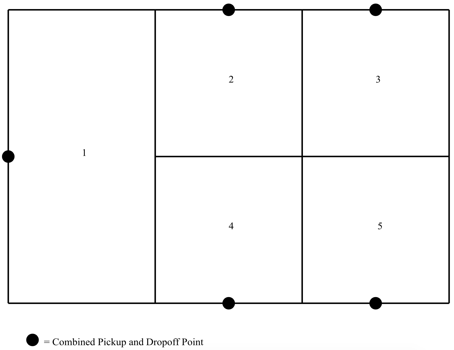
Consider the following manufacturing system described in Askin and Standridge (1993) and shown in Figure 17-5. There are five departments. Material movement between departments is performed using an AGV system.
Figure 17-5: AVG Path for Application Problem

Material flow volumes between departments per eight hour day are shown in the following table.
| From/To | 1 | 2 | 3 | 4 | 5 | Total From |
| 1 | 10 | 25 | 35 | |||
| 2 | 10 | 25 | 35 | |||
| 3 | 15 | 10 | 25 | |||
| 4 | 40 | 20 | 60 | |||
| 5 | 24 | 10 | 50 | 84 |
Note that each department uses the same point for dropoffs and pickups. AGV travel time is 3 feet/second. Assume that the sequence of interdepartmental moves is essentially random but that the time between move requests can be modeled as a constant value.
Each department is 30 feet by 30 feet in size except department 1 which is 30 feet by 60 feet. Pickup and dropoff times are 15 seconds.
The problem is to determine the routes taken by AGV's between each pair of stations. In addition, the number of AGV's required in this system as well as the effectiveness of the system as measured by the time from the request to move a load until load movement is completed must be determined. Both the average and maximum times are of interest.
If the AGV system as designed proves ineffective, it may be improved by moving pickup and dropoff points. The redesign could include having separate pickup and dropoff point. A new AGV path could be defined as well.
The simulation study should answer the following questions:
- Is one AGV sufficient for the current demand or are two AGV's necessary?
- If demand increases uniformly across all stations by 20%, what adjustments to the system are necessary?
Case Problem Issues
- Can the same model developed in this chapter be used as is or slightly modified to apply to the case problem? What would the modifications be?
- What alternative AGV paths should be considered?
- For each department, what pickup and dropoff point locations should be considered?
- Are there any other performance measures besides load movement time and AGV utilization that could be important?
- How will verification and validation evidence be obtained?
- What is the expected number of AGV's required?
- How will the arrival of load movement requests be modeled?


