5.5: Conditioning of Matrix Inversion

We are now in a position to address some of the issues that came up in Example 1 of Lecture 4, regarding the sensitivity of the inverse \(A^{-1}\) and of the solution \(x = A^{-1}b\) to perturbations in \(A\) (and/or \(b\), for that matter). We first consider the case where \(A\) is invertible, and examine the sensitivity of \(A^{-1}\). Taking differentials in the defining equation \(A^{-1}A = I\), we find

\[d\left(A^{-1}\right) A+A^{-1} d A=0 \ \tag{5.23}\]

where the order of the terms in each half of the sum is important, of course. (Rather than working with differentials, we could equivalently work with perturbations of the form \(A+\epsilon P\), etc., where \(\epsilon\) is vanishingly small, but this really amounts to the same thing.) Rearranging the preceding expression, we find

\[d\left(A^{-1}\right) = A^{-1} d A A^{-1} \ \tag{5.24}\]

Taking norms, the result is

\[\left\|d\left(A^{-1}\right)\right\| \leq\left\|A^{-1}\right\|^{2}\|d A\| \ \tag{5.25}\]

or equivalently

\[\frac{\left\|d\left(A^{-1}\right)\right\|}{\left\|A^{-1}\right\|} \leq\|A\|\left\|A^{-1}\right\| \frac{\|d A\|}{\|A\|} \ \tag{5.26}\]

This derivation holds for any submultiplicative norm. The product \(\|A\|\left\|A^{-1}\right\|\) is termed the condition number of \(A\) with respect to inversion (or simply the condition number of \(A\)) and denoted by \(K(A)\):

\[K(A) = \|A\|\left\|A^{-1}\right\| \ \tag{5.27}\]

When we wish to specify which norm is being used, a subscript is attached to \(K(A)\). Our earlier results on the SVD show, for example, that

\[K_{2}(A)=\sigma_{\max } / \sigma_{\min } \ \tag{5.28}\]

The condition number in this 2-norm tells us how slender the ellipsoid \(Ax\) for \(\|x\|_{2}=1\) is - see Figure 5.1. In what follows, we shall focus on the 2-norm condition number (but will omit the subscript unless essential).

Some properties of the 2-norm condition number (all of which are easy to show, and some of which extend to the condition number in other norms) are

• \(K(A) \geq 1;\)
• \(K(A) = K(A^{-1});\)
• \(K(AB) \leq K(A) K(B);\)
• Given \(U^{\prime}U = I\), \(K(UA) = K(A)\).

The importance of (5.26) is that the bound can actually be attained for some choice of the perturbation \(dA\) and of the matrix norm, so the situation can get as bad as the bound allows: the fractional change in the inverse can be \(K(A)\) times as large as the fractional change in the original. In the case of 2-norms, a particular perturbation that attains the bound

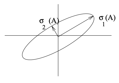
Figure \(\PageIndex{1}\): Depiction of how A (a real \(2 \times 2\) matrix) maps the unit circle. The major axis of the ellipse corresponds to the largest singular value, the minor axis to the smallest.

can be derived from the \(\Delta\) of Theorem 5.1, by simply replacing \(-\sigma_{n}\) in \(\Delta\) by a differential perturbation:

\[d A=-d \sigma u_{n} v_{n}^{\prime} \ \tag{5.29}\]

We have established that a large condition number corresponds to a matrix whose inverse is very sensitive to relatively small perturbations in the matrix. Such a matrix is termed ill conditioned or poorly conditioned with respect to inversion. A perfectly conditioned matrix is one whose condition number takes the minimum possible value, namely 1.

A high condition number also indicates that a matrix is close to losing rank, in the following sense: There is a perturbation \(\Delta\) of small norm (\(=\sigma_{min}\)) relative to \(\|A\|\left(=\sigma_{\max }\right)\) such that \(A + \Delta\) has lower rank than \(A\). This follows from our additive perturbation result in Theorem 5.1. This interpretation extends to non-square matrices as well. We shall term the ratio in (5.28) the condition number of \(A\) even when \(A\) is non-square, and think of it as a measure of nearness to a rank loss.

Turning now to the sensitivity of the solution \(x = A^{-1}b\) of a linear system of equations in the form \(Ax = b\), we can proceed similarly. Taking differentials, we find that

\[d x=-A^{-1} d A A^{-1} b+A^{-1} d b=-A^{-1} d A x+A^{-1} b \ \tag{5.30}\]

Taking norms then yields

\[\|d x\| \leq\left\|A^{-1}\right\|\|d A\|\|x\|+\left\|A^{-1}\right\|\|d b\| \ \tag{5.31}\]

Dividing both sides of this by \(\|x\|\), and using the fact that \(\|x\| \geq (\|b\|/\|A\|)\), we get

\[\frac{\|d x\|}{\|x\|} \leq K(A)\left(\frac{\|d A\|}{\|A\|}+\frac{\|d b\|}{\|b\|}\right) \ \tag{5.32}\]

We can come close to attaining this bound if, for example, \(b\) happens to be nearly collinear with the column of \(U\) in the SVD of \(A\) that is associated with \(\sigma_{min}\), and if appropriate perturbations occur. Once again, therefore, the fractional change in the answer can be close to \(K(A)\) times as large as the fractional changes in the given matrices.

Example 5.2

For the matrix A given in Example 1 of Lecture 4, the SVD is

\[A=\left(\begin{array}{cc}
100 & 100 \\
100.2 & 100
\end{array}\right)=\left(\begin{array}{cc}
.7068 & .7075 \\
.7075 & .-7068
\end{array}\right)\left(\begin{array}{cc}
200.1 & 0 \\
0 & 0.1
\end{array}\right)\left(\begin{array}{cc}
.7075 & .7068 \\
-.7068 & .7075
\end{array}\right) \ \tag{5.33}\]

The condition number of \(A\) is seen to be 2001, which accounts for the 1000-fold magnification of error in the inverse for the perturbation we used in that example. The perturbation \(\Delta\) of smallest 2-norm that causes \(A + \Delta\) to become singular is

\[\Delta=\left(\begin{array}{cc}
.7068 & .7075 \\
.7075 & .-7068
\end{array}\right)\left(\begin{array}{cc}
0 & 0 \\
0 & -0.1
\end{array}\right)\left(\begin{array}{cc}
.7075 & .7068 \\
-.7068 & .7075
\end{array}\right)\nonumber\]

whose norm is 0.1. Carrying out the multiplication gives

\[\Delta \approx\left(\begin{array}{cc}
.05 & -.05 \\
-.05 & .05
\end{array}\right)\nonumber\]

With \(b = [1 - 1]^{T}\), we saw large sensitivity of the solution \(x\) to perturbations in \(A\). Note that this \(b\) is indeed nearly collinear with the second column of \(U\). If, on the other hand, we had \(b=\left[\begin{array}{ll}
1 & 1
\end{array}\right]\), which is more closely aligned with the first column of \(U\), then the solution would have been hardly affected by the perturbation in \(A\) - a claim that we leave you to verify.

Thus \(K(A)\) serves as a bound on the magnification factor that relates fractional changes in \(A\) or \(b\) to fractional changes in our solution \(x\).

Conditioning of Least Squares Estimation

Our objective in the least-square-error estimation problem was to find the value \(\widehat{x}\) of \(x\) that minimizes \(\|y-A x\|_{2}^{2}\), under the assumption that \(A\) has full column rank. A detailed analysis of the conditioning of this case is beyond our scope (see Matrix Computations by Golub and Van Loan, cited above, for a detailed treatment). We shall make do here with a statement of the main result in the case that the fractional residual is much less than 1, i.e.

\[\frac{\|y-A \widehat{x}\|_{2}}{\|y\|_{2}} \ll 1 \ \tag{5.34}\]

This low-residual case is certainly of interest in practice, assuming that one is fitting a reasonably good model to the data. In this case, it can be shown that the fractional change \(\|d \widehat{x}\|_{2} /\|\widehat{x}\|_{2}\) in the solution \(\widehat{x}\) can approach \(K(A)\) times the sum of the fractional changes in \(A\) and \(y\), where \(K(A)=\sigma_{\max }(A) / \sigma_{\min }(A)\). In the light of our earlier results for the case of invertible \(A\), this result is perhaps not surprising.

Given this result, it is easy to explain why solving the normal equations

\[\left(A^{\prime} A\right) \widehat{x}=A^{\prime} y\nonumber\]

to determine \(\widehat{x}\) is numerically unattractive (in the low-residual case). The numerical inversion of \(A^{\prime}A\) is governed by the condition number of \(A^{\prime}A\), and this is the square of the condition number of \(A\):

\[K\left(A^{\prime} A\right)=K^{2}\tag{A}\]

You should confirm this using the SVD of \(A\). The process of directly solving the normal equations will thus introduce errors that are not intrinsic to the least-square-error problem, because this problem is governed by the condition number \(K(A)\), according to the result quoted above. Fortunately, there are other algorithms for computing \(\widehat{x}\) that are governed by the condition number \(K(A)\) rather than the square of this (and Matlab uses one such algorithm to compute \(\widehat{x}\) when you invoke its least squares solution command).