5.5: Transient and Steady-State Improvement
- Page ID
- 28539

Lead–Lag and PID Designs
When control system design specifications require simultaneous improvement to the transient response and the steady-state tracking error, a lead-lag or a PID controller may be considered.
A lead-lag controller combines phase-lead and phase-lag stages; as a rule, the the transient response is improved first, followed by steady-state error improvement. The lead-lag controller is expressed as:
\[K(s)=K\left(\frac{s+z_{\rm c1}}{s+p_{\rm c1}}\right)\left(\frac{s+z_{\rm c2}}{s+p_{\rm c2}}\right),\quad z_{\rm c1}<p_{\rm c1}, \; z_{\rm c2}>p_{\rm c2} \nonumber \]
a PID controller similarly combines PD and PI controllers. It is expressed as:
\[K(s)=K\left({s+z_{\rm c1}}\right)\left(\frac{s+z_{\rm c2}}{s}\right) \nonumber \]
As a rule, the transient response improvement is aimed first. The pole and zero selected for phase-lead or PD design steer the root locus toward the desired closed-loop pole locations. The pole-zero pair in the phase-lag or PI part of the design is located close to the origin in order to minimally disturb the existing root locus.
Lead-Lag Design
Let \(G\left(s\right)=\frac{10}{s\left(s+2\right)(s+5)}\); assume that the design specifications are: \(\% {\rm O}S\le 10\% ,\; \; t_\rm s \le 2\rm s,\; \; e_{\rm ss} |_{{\rm r}amp} \le 0.1.\) These specifications translate into: \(\zeta \ge 0.6,\ \sigma \ge 2,\ K_v\ge 10\).
Phase-Lead Design. The phase-lead controller design (covered in Example 5.3.3) proceeds as follows: Let \(s_1=-2.2\pm j2.4,\;\;\zeta =0.68,\) denote a desired closed-loop pole location; then, \(G\left(s_1\right)=0.35\angle 92{}^\circ\), i.e., the required controller phase contribution is: \(K\left(s_1\right)=K\angle 88{}^\circ\).
Let \(z_c=2,\ p_c=22\); then \(K\left(s_1\right)=0.11\angle 88{}^\circ\). From the RL plot, a controller gain \(K=24\) is selected for closed-loop roots at: \(s=-2.2\pm j2.4\). Hence, the phase-lead section is designed as: \(K_{\rm lead}\left(s\right)=24\left(\frac{s+2}{s+22}\right)\).
Phase-lag Design. For \(K_{\rm lead} (s)G(s)\), the velocity error constant is given as: \(K_v=2.2\). To boost the error constant to \(K_v>10\), a phase-lag controller, \(K_{\rm lag}=\frac{s+0.01}{s+0.002}\) is considered.
The angle contribution of the phase-lag controller is: \(\angle K_{\rm lag}\left(s_1\right)=-0.1{}^\circ\) hence the dominant closed-loop roots are negligibly affected.
The lead-lag controller is formed as: \(K\left(s\right)=25\left(\frac{s+2}{s+24}\right)\left(\frac{s+0.01}{s+0.002}\right)\).
The closed-loop transfer function is obtained as: \(T\left(s\right)=\frac{240\left(s+0.01\right)}{\left(s+0.01004\right)\left(s+22.6\right)\left(s^2+4.39s+10.58\right)}\). The dominant closed-loop roots are located at: \(s=-2.2\pm j2.4\ (\zeta =0.68)\).
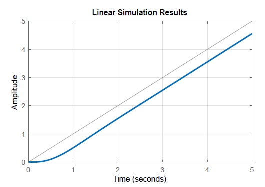
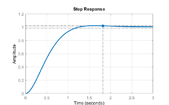
The step and ramp responses of the closed-loop system are plotted below. The step response displays a settling time of \(1.9sec\).
PID Design
An alternate PID design is performed in the next example.
Let \(G\left(s\right)=\frac{10}{s\left(s+2\right)(s+5)}\); assume that the design specifications are: \(\% {\rm O}S\le 10\% ,\; \; t_\rm s \le 2\rm s,\; \; e_{\rm ss} |_{{\rm r}amp} \le 0.1.\) These specifications translate into: \(\zeta \ge 0.6,\ \sigma \ge 2,\ K_v\ge 10\).
PD design. The PD controller is given as: \(K_{PD}\left(s\right)=K\left(s+z_c\right)\). We may arbitrarily choose the controller zero at \(z_c=-2\), and use the root locus of the compensated system to select \(K=1\) with closed-loop roots at: \(s_1=-2.5\pm j1.95\).
PI design. The PI controller is given as: \(\frac{s+z_c}{s}\), where \(z_c\ll s_1\) is desired. We may arbitrarily select a zero location: \(z_c=0.01\) to define the PID controller as: \(K_{PID}\left(s\right)=\frac{(s+0.01)(s+2)}{s}\).
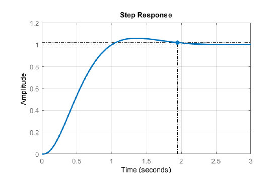
The closed-loop transfer function is given as: \(T\left(s\right)=\frac{10\left(s+0.01\right)}{\left(s+0.01005\right)\left(s+2\right)\left(s^2+4.99s+9.95\right)}\).
The step response of the closed-loop system shows a settling time of \(t_s=1.8sec\).
Phase-Lead with PI
We can also combine the phase-lead controller design with a PI controller to define the composite controller as shown below.
Let \(G\left(s\right)=\frac{10}{s\left(s+2\right)(s+5)}\); assume that the design specifications are: \(\% {\rm O}S\le 10\% ,\; \; t_\rm s \le 2\rm s,\; \; e_{\rm ss} |_{\rm ramp} \le 0.1.\) These specifications translate into: \(\zeta \ge 0.6,\ \sigma \ge 2,\ K_v\ge 10\).
Phase-Lead Design. Let \(s_1=-2.2\pm j2.4\,\;\;\zeta =0.68\); then, we may choose, as in Example 5.5.1 above, \(z_c=2,\ p_c=22\) and \(K=24\) for closed-loop roots at: \(s=-2.2\pm j2.4\). The phase-lead controller is defined as: \(K_{\rm lead}\left(s\right)=24\left(\frac{s+2}{s+22}\right)\).
PI design. The PI controller is given as: \(\frac{s+z_c}{s}\). In this case, \(z_c=0.01\) does not appear to be a good choice, as the slow mode in the step response remains dominant, increasing the settling time.
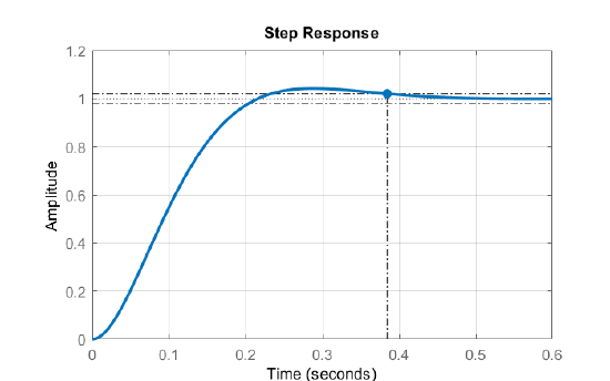
A better strategy is to select the PI controller zero to cancel the second plant pole at \(s=-5\). The composite controller is formed as: \(K\left(s\right)=24\left(\frac{s+2}{s+22}\right)\left(\frac{s+5}{s}\right)\).
The resulting closed-loop transfer function after pole-zero cancelations is given as: \(T\left(s\right)=\frac{240}{\left(s^2+22s+240\right)}\), which has dominant closed-loop roots located at: \(s=-11\pm j11\ (\zeta =0.7)\).
The step response of the closed-loop system shows a short settling time of \(t_s\cong 0.38sec\).
MATLAB Tuning of PID Controller
The MATLAB Control Systems Toolbox offers the ‘pidtune’ command to design an optimal PID controller or a PID controller with a filter to reduce high frequency noise.
Let \(G\left(s\right)=\frac{10}{s\left(s+2\right)(s+5)}\); then, the MATLAB tuned PID controller is obtained as:
\[K\left(s\right)=\frac{2.01\left(s+0.314\right)\left(s+1.43\right)}{s} \nonumber \]
The resulting closed-loop roots are located at: \(s=-0.34,\ -1.16,\ -2.73\pm 3.71.\)
Alternatively, MATLAB tuned PID controller with filter is obtained as:
\[K\left(s\right)=\frac{727.25\left(s+0.302\right)\left(s+1.41\right)}{s\left(s+361.4\right)} \nonumber \]
The resulting closed-loop roots are located at: \(s=-0.34,\ -1.16,\ -2.73\pm 3.71,\ -361.5.\)
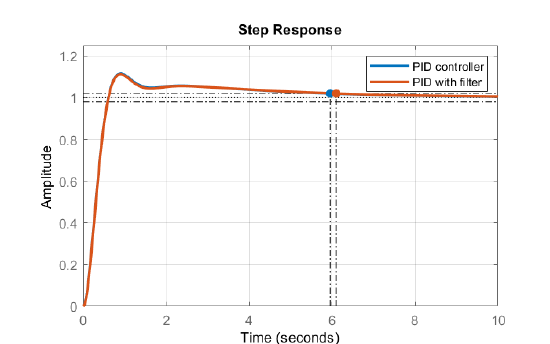
The closed-loop system responses for the MATLAB designed PID controllers are plotted below. The responses are almost identical with an overshoot of about \(10\%\) with a settling time of \(t_s\cong 6sec\).