6.1: Frequency Response Plots
- Page ID
- 24413

Frequency Response Function
The frequency response of the loop transfer function, \(KGH(s)\), is represented as: \(KGH(j\omega )=\left. KGH(s)\right|_{s=j\omega }\).
For a particular value of \(\omega\), the \(KGH(j\omega )\) is a complex number, which is described in terms of its magnitude and phase as \(KGH(j\omega )=|KGH(j\omega )|e^{j\phi (\omega )}\).
As \(\omega\) varies from \(0\) to \(\infty\), \(KGH(j\omega )\) can be plotted in the complex plane (the polar plot). Alternatively, both magnitude and phase can be plotted as functions of \(\omega\) (the Bode magnitude and phase plots).
Bode Plot
To proceed further, we assume that the loop transfer function is expressed using first and second order factors as:
\[KGH(s)=\frac{K\prod _{i=1}^{m} \left(1+\frac{s}{z_{i} } \right)}{s^{n_{0} } \prod _{i=1}^{n_{1} } \left(1+\frac{s}{p_{i} } \right)\prod _{i=1}^{n_{2} } \left(1+2\zeta _{i} \frac{s}{\omega _{n,i} } +\frac{s^{2} }{\omega _{n,i}^{2} } \right)} \nonumber \]
where \(m\) is the number of real zeros, \(n_0\) is the number of poles at the origin, \(n_1\) is the number of real poles, \(n_2\) is the number of complex pole pairs, and \(K\) is a scalar gain. Further, \(z_i\) and \(p_i\) represent the zero and pole frequencies for first-order factors; \(\omega _{n,i}\) and \(\zeta _i\) represent the natural frequency and damping ratio of second-order factors.
The corresponding frequency response function is given as:
\[KGH(j\omega )=\frac{K\prod _{i=1}^{m} \left(1+j\frac{\omega }{z_{i} } \right)}{(j\omega )^{n_{0} } \prod _{i=1}^{n_{1} } \left(1+j\frac{\omega }{p_{i} } \right)\prod _{i=1}^{n_{2} } \left(1-\frac{\omega ^{2} }{\omega _{n,i}^{2} } +j2\zeta _{i} \frac{\omega }{\omega _{n,i} } \right)} \nonumber \]
It is customary to plot the magnitude of the frequency response function on the log scale as \(|G(j\omega )|_{\rm dB} =20\; \log _{10} |G(j\omega )|\). The magnitude of the loop gain is given in dB as:
\[\begin{array}{r} {|KGH(j\omega )|_{\rm dB} =20\; \log K+\sum _{i=1}^{m} 20\; \log \left|1+\frac{j\omega }{z_{i} } \right|-(20n_{0} )\log \omega } \\ {-\sum _{i=1}^{n_{1} } 20\; \log \left|1+\frac{j\omega }{p_{i} } \right|-\sum _{i=1}^{n_{2} } 20\; \log \left|1-\frac{\omega ^{2} }{\omega _{n,i}^{2} } +j2\zeta _{i} \frac{\omega }{\omega _{n,i} } \right|.} \end{array} \nonumber \]
At low frequencies, the frequency response magnitude is a constant, i.e., \(\lim_{\omega\to 0} |KGH(j\omega )|_{\rm dB} =20\; \log K\).
For large \(\omega\), the magnitude plot is characterized by a slope: \(-20(n-m)\)dB/decade of \(\omega\), where \(n-m\) represents the pole excess of the loop transfer function.
The phase angle \(\phi (\omega )\) of the loop transfer function is computed as:
\[\phi (\omega )=\sum _{i=1}^{m} \angle \left(1+\frac{j\omega }{z_{i} } \right)-n_{0} (90^{\circ } )-\sum _{i=1}^{n_{1} } \angle \left(1+\frac{j\omega }{p_{i} } \right)-\sum _{i=1}^{n_{1} } \angle \left(1-\frac{\omega ^{2} }{\omega _{n,i}^{2} } +j2\zeta _{i} \frac{\omega }{\omega _{n,i} } \right). \nonumber \]
The phase angle for large \(\omega\) is given as: \(\phi (\omega )=-90^{\circ } (n-m)\).
In the MATLAB Control Systems Toolbox, the Bode plot is obtained by using the 'bode' command, which is invoked after defining the transfer function object.
Nyquist Plot
The frequency response function \(KGH(j\omega )\) represents a complex rational function of \(\omega\). The function can be plotted in the complex plane. A polar plot describes the graph of \(KGH(j\omega )\) \(\omega\) varies from \(0\to \infty\).
The Nyquist plot is a closed curve that describes a graph of \(KGH(j\omega )\) for \(\omega \in \left(-\infty ,~\infty \right)\). In the MATLAB Control Systems Toolbox the Nyquist plot is obtained by invoking the ‘nyquist’ command, invoked after defining the transfer function.
The shape of the Nyquist plot depends on the poles and zeros of \(KGH(j\omega )\); it can be pictured by estimating magnitude and phase of \(KGH(j\omega )\) at low and high frequencies. For example, if \(KGH(s)\) has no poles at the origin, then at low frequency, \(KGH(j0)\cong K\angle 0^{\circ }\); while, at high frequency, \(|KGH(j\infty )|\to 0\), and\(\angle KGH(j\infty )=-90^{\circ } (n-m)\), where \(n-m\) represents the pole excess of \(KGH(s)\).
In particular, for \(n-m=3\), the Nyquist plot crosses the negative real-axis at the phase crossover frequency, \({\omega }_{pc}\). Let \(G\left(j{\omega }_{pc}\right)=g\angle 180{}^\circ\); then, the gain margin is given as \(g^{-1}\). Further, for \(K=g^{-1}\), the Nyquist plot of \(KG\left(j\omega \right)\) passes through the \(-1+j0\), described as the critical point for stability determination.
The number of unstable closed-loop poles of \(\Delta (s)=1+KGH(s)\) equals the number of unstable open-loop poles of \(KGH(s)\)plus the number of clock-wise (CW) encirclements of the \(-1+j0\) point on the complex plane by the Nyquist plot of \(KGH(s)\).
Examples
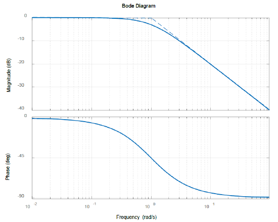
Let \(G(s)=\frac{1}{s+1}\); then, \(G(j\omega )=\frac{1}{1+j\omega } =\frac{1}{\sqrt{1+\omega ^{2} } } \; \angle -\tan ^{-1} \omega\).
In particular, at specific points, \(G(j0)=1\; \angle 0^{\circ }\), \(G\left(j1\right)=\frac{1}{\sqrt{2}}\angle -45{}^\circ\), and \(G(j\infty )=0\; \angle -90^{\circ }\).
The Bode magnitude plot (Figure 6.1.1) starts at \(0\ dB\) with an initial slope of zero that gradually changes to \(-20\ dB\) per decade at high frequencies. An asymptotic Bode plot consists of two lines joining ar the corner frequency (1 rad/s).
The Bode phase plot varies from \(0{}^\circ\) to \(-90{}^\circ\) with a phase of \(\ -45{}^\circ\) at the corner frequency.
The Nyquist plot of \(G\left(s\right)\) is circle in the right-half plane (RHP). Further, for \(K>0\), the Nyquist plot of \(KG\left(j\omega \right)\) is confined to the RHP; hence, by Nyquist stability criterion, the closed-loop system is stable for all \(K>0\).
Let \(G(s)=\frac{1}{s(s+1)}\); then, \(G(j\omega )=\frac{1}{j\omega (1+j\omega )} =\frac{1}{\omega } \frac{1}{\sqrt{1+\omega ^{2} } } \angle -90^{\circ } -\tan ^{-1} \omega \).
In particular, \(G\left(j0\right)=\infty \angle -90{}^\circ\), \(G\left(j1\right)=\frac{1}{\sqrt{2}}(-3dB)\angle -135{}^\circ\), \(G\left(j\infty \right)=0\angle -180{}^\circ\).
The Bode magnitude plot (Figure 6.1.2) has an initial slope of \(-20\ dB\) per decade that gradually changes to \(-40\ dB\) per decade at high frequencies. The phase plot shows a variation from \(-90{}^\circ\) to \(-180{}^\circ\) with a phase of \(\ -135{}^\circ\) at the corner frequency.
The Nyquist plot is a closed curve that travels along negative \(j\omega\)-axis for \(\omega \in (0,\infty )\), along positive \(j\omega\)-axis for \(\omega \in (-\infty ,0)\), and scribes a semi-circle of a large radius for \(\omega \in \left(0^-,0^+\right)\). As the Nyquist plot of \(KG\left(j\omega \right)\) stays away from the critical point (\(-1+j0\)) for positive values of \(K\), the closed-loop system is projected to be stable for all \(K>0\).
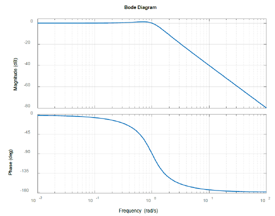
Let \(G\left(s\right)=\frac{1}{s^2+s+1}\); then, \(G\left(j\omega \right)=\frac{1}{1-{\omega }^2+j\omega }=\frac{1}{\sqrt{\left(1-{\omega }^2\right)^2+\left(\omega \right)^2}} \angle -{tan}^{-1} \frac{\omega }{1-{\omega }^2}\).
In particular, \(G\left(j0\right)=1\left(0dB\right)\angle 0{}^\circ\), \(G\left(j1\right)=1\left(0dB\right)\angle -90{}^\circ\), \(G\left(j\infty \right)=0\angle -180{}^\circ\).
The Bode magnitude plot (Figure 6.1.3) starts at \(0\ dB\) with an initial slope of 0; the slope changes to \(-40\ dB\) per decade for \(\omega >1\). The magnitude plot shows a resonance peak at the corner frequency due to the low value of \(\zeta=0.5\).
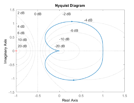
The Nyquist plot of \(G\left(j\omega \right)\) is a closed curve that has no crossing with the negative real-axis. As the Nyquist plot of \(KG\left(j\omega \right),\ K>0\) stays away from the critical point (\(-1+j0\)), the closed-loop system is projected to be stable for all \(K>0\).
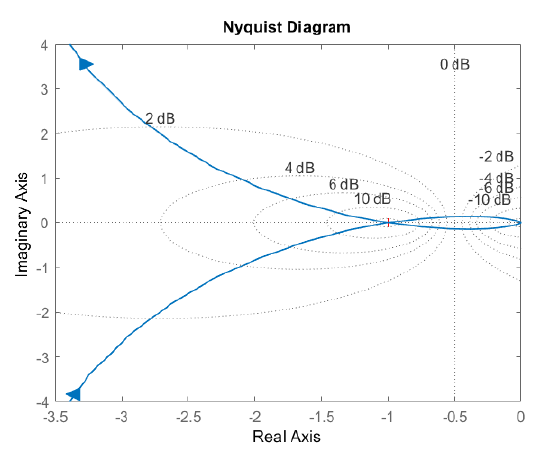
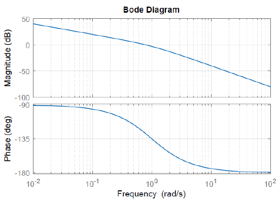
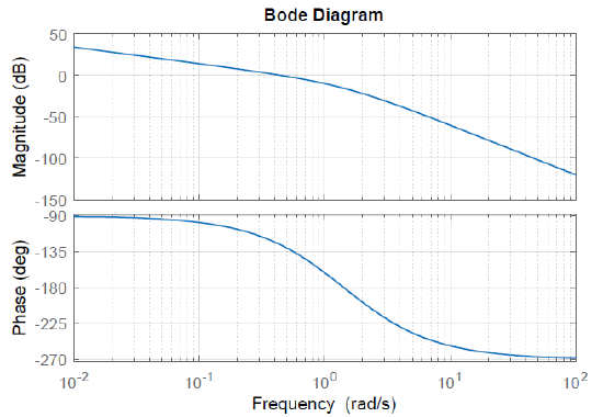
Let \(G(s)=\frac{2}{s(s+1)(s+2)}\); then, \(G(j\omega )=\frac{2}{j\omega (1+j\omega )(2+j\omega )} =\frac{1}{\omega } \frac{1}{\sqrt{1+\omega ^{2} } } \frac{2}{\sqrt{2+\omega ^{2} } } \; \angle -90^{\circ } -\tan ^{-1} \omega -\tan ^{-1} 2\omega . \nonumber\).
In particular, \(G\left(j0\right)=\infty \angle -90{}^\circ\), \(G\left(j1\right)=\frac{2}{\sqrt{10}}\left(-4dB\right)\angle -108{}^\circ\), \(G\left(j1\right)=\frac{1}{5\sqrt{2}}\left(-13dB\right)\angle -139{}^\circ\), and \(G\left(j\infty \right)=0dB\angle -270{}^\circ\).
The Bode magnitude plot (Figure 6.1.4) has an initial slope of \(-20\ dB\) per decade that changes first to \(-40\ dB\) per decade and then to \(-60\ dB\)/decade at high frequencies. The phase plot shows a variation from \(-90{}^\circ\) to \(-270{}^\circ\).
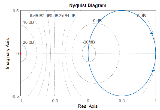
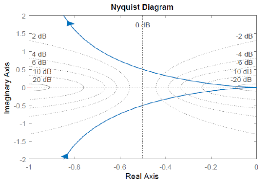
The polar plot begins with a large magnitude along the negative \(j\omega\)-axis (for \(\omega =0^+\)), crosses the negative real-axis at \(0.33\angle 180{}^\circ\) (for \(\omega =3.32\)), and approaches the origin from the positive \(j\omega\)-axis (for \(\omega \to\infty\)).
The Nyquist plot, obtained by joining a reflection of the polar plot, includes a closed contour that includes a negative real-axis crossing at \(0.33\angle 180{}^\circ\). As the plot expands for \(K>1\), it encloses the critical (\(-1+j0\)) point. The closed-loop system is projected to be stable for \(K<3\).
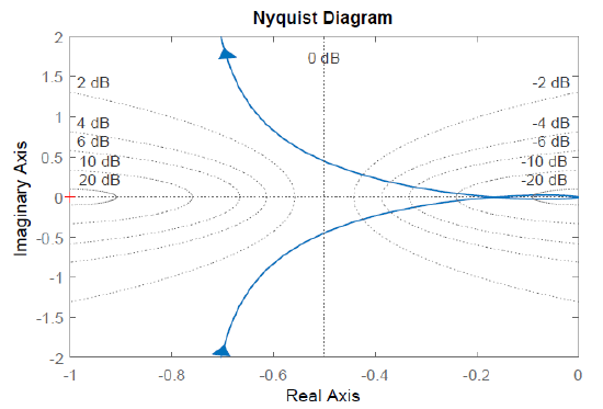
Further, the Nyquist plot for \(K=3\) passes through the critical point.
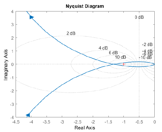
The Nyquist plot for \(K=4\) crosses the real axis to the left of the critical point as shown in the figure below. In addition, the plot of \(KGH(j\omega)\) for \(s\in(0^-,0^+)\) subscribes a large circle in the complex plane (not shown in the figure). Hence the Nyquist plot completes two CW encirclements of the critical point, indicating two unstable closed-loop roots.