2.4: Analogies

Because abstractions are so useful, it is helpful to have methods for making them. One way is to construct an analogy between two systems. Each common feature leads to an abstraction; each abstraction connects our knowledge in one system to our knowledge in the other system. One piece of knowledge does double duty. Like a mental lever, analogy and, more generally, abstraction are intelligence amplifiers.

2.4.1 Electrical–mechanical analogies

An illustration with many abstractions on which we can practice is the analogy between a spring–mass system and an inductor–capacitor (LC) circuit.

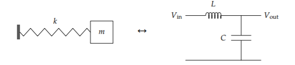
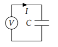
In the circuit, the voltage source—the V_in on its left side—supplies a current that flows through the inductor (a wire wrapped around an iron rod) and capacitor (two metal plates separated by air). As current flows through the capacitor, it alters the charge on the capacitor. This “charge” is confusingly named, because the net charge on the capacitor remains zero. Instead, “charge” means that the two plates of the capacitor hold opposite charges, Q and -Q, with Q ≠ 0. The current changes Q. The charges on the two plates create an electric field, which produces the output voltage V out equal to Q/C (where C is the capacitance).

For most of us, the circuit is less familiar than the spring–mass system. However, by building an analogy between the systems, we transfer our understanding of the mechanical to the electrical system.

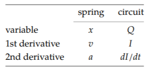
In the mechanical system, the fundamental variable is the mass's displacement x. In the electrical system, it is the charge Q on the capacitor. These variables are analogous so their derivatives should also be analogous: velocity (v), the derivative of position, should be analogous to current (I), the derivative of charge.

Let’s build more analogy bridges. The derivative of velocity, which is the second derivative of position, is acceleration (a). Therefore, the derivative of current (dI/dt) is the analog of acceleration. This analogy will be useful shortly when we find the circuit’s oscillation frequency.

These variables describe the state of the systems and how that state changes: They are the kinematics. But without the causes of the motion—the dynamics—the systems remain lifeless. In the mechanical system, dynamics results from force, which produces acceleration:

\[a = \frac{F}{m}\]

Acceleration is analogous to change in current dI/dt, which is produced by applying a voltage to the inductor. For an inductor, the governing relation (analogous to Ohm’s law for a resistor) is

\[\frac{dI}{dt} = \frac{V}{L}\]

where L is the inductance, and V is the voltage across the inductor. Based on the common structure of the two relations, force F and voltage V must be analogous. Indeed, they both measure effort: Force tries to accelerate the mass, and voltage tries to change the inductor current. Similarly, mass and inductance are analogous: Both measure resistance to the corresponding effort. Large masses are hard to accelerate, and large-L inductors resist changes to their current. (A mass and an inductor, in another similarity, both represent kinetic energy: a mass through its motion, and an inductor through the kinetic energy of the electrons making its magnetic field.)

Turning from the mass–inductor analogy, let’s look at the spring–capacitor analogy. These components represent the potential energy in the system: in the spring through the energy in its compression or expansion, and in the capacitor through the electrostatic potential energy due to its charge.

Force tries to stretch the spring but meets a resistance k: The stiffer the spring (the larger its k), the harder it is to stretch.

\[x = \frac{F}{k}\]

Analogously, voltage tries to charge the capacitor but meets a resistance 1/C: The larger the value of 1/C, the smaller the resulting charge.

\[Q = \frac{V}{1/C}\]

Based on the common structure of the relations for x and Q, spring constant k must be analogous to inverse capacitance 1/C. Here are all our analogies.

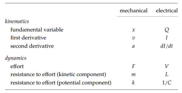
From this table, we can read off our key result. Start with the natural (angular) frequency \(\omega\) of a spring–mass system: \(\omega = \frac{k}{m}\) Then apply the analogies. Mass m is analogous to inductance L. Spring constant k is analogous to inverse capacitance 1/C. Therefore, \(\omega\) for the LC circuit is 1/LC :

\[\omega = \sqrt\frac{1/C}{L} = \frac{1}{\sqrt{LC}}\]

Because of the analogy bridges, one formula, the natural frequency of a spring–mass system, does double duty. More generally, whatever we learn about one system helps us understand the other system. Because of the analogies, each piece of knowledge does double duty.

2.4.2 Energy density in the gravitational field

With the electrical–mechanical analogy as practice, let’s try a less familiar analogy: between the electric and the gravitational field. In particular, we’ll connect the energy densities (energy per volume) in the corresponding fields. An electric field E represents an energy density of \(\epsilon_{0}E^{2}/2\), where \(\epsilon_{0}\) is the permittivity of free space appearing in the electrostatic force between two charges q₁ and q₂:

\[F = \frac{q_{1}q_{2}}{4 \pi \epsilon_{0} r^{2}}\]

Because electrostatic and gravitational forces are both inverse-square forces (the force is proportional to 1/r²), the energy densities should be analogous. Not least, there should be a gravitational energy density. But how is it related to the gravitational field?

To answer that question, our first step is to find the gravitational analog of the electric field. Rather than thinking of the electric field only as something electric, focus on the common idea of a field. In that sense, the electric field is the object that, when multiplied by the charge, gives the force:

\[\textrm{force = charge} \times \textrm{field}\]

We use words rather than the normal symbols, such as E for field or q for charge, because the symbols might bind our thinking to particular cases and prevent us from climbing the abstraction ladder.

This verbal form prompts us to ask: What is gravitational charge? In electrostatics, charge is the source of the field. In gravitation, the source of the field is mass. Therefore, gravitational charge is mass. Because field is force per charge, the gravitational field strength is an acceleration:

\[gravitational \: field = \frac{force}{charge} = \frac{force}{mass} = acceeration\]

Indeed, at the surface of the Earth, the field strength is g, also called the acceleration due to gravity.

The definition of gravitational field is the first half of the puzzle (we are using divide-and-conquer reasoning again). For the second half, we’ll use the field to compute the energy density. To do so, let’s revisit the route from electric field to electrostatic energy density:

\[E \rightarrow \frac{1}{2} \epsilon_{0} E^{2}\]

With g as the gravitational field, the analogous route is

\[g \rightarrow \frac{1}{2} \times somethings \times g^{2}\]

where the “something” represents our ignorance of what to do about \(\epsilon_{0}\).

What is the gravitational equivalent of \(\epsilon_{0}\)?

To find its equivalent, compare the simplest case in both worlds: the field of a point charge. A point electric charge q produces a field

\[E = \frac{1}{4 \pi \epsilon_{0}}\frac{q}{r^{2}}\]

A point gravitational charge m (a point mass) produces a gravitational field (an acceleration)

\[g = \frac{Gm}{r^{2}}\]

where G is Newton's constant.

The gravitational field has a similar structure to the electric field. Both are inverse-square forces, as expected. Both are proportional to the charge. The difference is the constant of proportionality. For the electric field, it is \(\frac{1}{4 \pi \epsilon_{0}}\). For the gravitational field, it is simply G. Therefore, G is analogous to \(\frac{1}{4 \pi \epsilon_{0}}\); equivalently, \(\epsilon_{0}\) is analogous to \(\frac{1}{4 \pi G}\).

Then the gravitational energy density becomes

\[\frac{1}{2} \times \frac{1}{4 \pi G} \times g^{2} = \frac{g^{2}}{8 \pi G}\]

We will use this analogy in Section 9.3.3 when we transfer our hard-won knowledge of electromagnetic radiation to understand the even more subtle physics of gravitational radiation.

Exercise \(\PageIndex{1}\): Gravitational energy of the Sun

What is the energy in the gravitational field of the Sun? (Just consider the field outside the Sun.)

Exercise \(\PageIndex{2}\): Pendulum period including buoyancy

The period of a pendulum in vacuum is (for small amplitudes) \(T = 2 \pi \sqrt \frac{l}{g}\), where l is the bob length and g is the gravitational field strength. Now imagine the pendulum swinging in a fluid (say, air). By replacing g with a modified value, include the effect of buoyancy in the formula for the pendulum period.

Exercise \(\PageIndex{3}\): Comparing field energies

Find the ratio of electrical to gravitational field energies in the fields produced by a proton.

2.4.3 Parallel combination

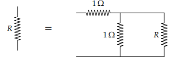
Analogies not only reuse work, they help us rewrite expressions in compact, insightful forms. An example is the idea of parallel combination. It appears in the analysis of the infinite resistive ladder of Problem 2.8.

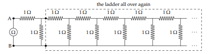
To find the resistance R across the ladder (in other words, what the ohmmeter measures between the nodes A and B), you represent the entire ladder as a single resistor R. Then the whole ladder is 1 ohm in series with the parallel combination of 1 ohm and R:

The next step in finding R usually invokes the parallel-resistance formula: that the resistance of R₁ and R₂ in parallel is

\[\frac{R_{1}R_{2}}{R_{1} + R_{2}}\]

For our resistive ladder, the parallel combination of 1 ohm with the ladder is 1 ohm × R/(1 ohm + R). Placing this combination in series with 1 ohm gives a resistance

\[1 \Omega + \frac{1 \Omega \times R}{1 \Omega + R}\]

This recursive construction reproduces the ladder, only one unit longer. We therefore get an equation for R:

\[R = 1 \Omega + \frac{1 \Omega \times R}{1 \Omega + R}\]

The (positive) solution is \(R = (1 + \sqrt 5 )/2\) ohms. The numerical part is the golden ratio \(\phi\) (approximately 1.618). Thus, the ladder, when built with 1-ohm resistors, offers a resistance of \(\phi\) ohms.

Although the solution is correct, it skips over a reusable idea: the parallel combination. To facilitate its reuse, let’s name the idea with a notation:

\[R_{1} \parallel R_{2}\]

This notation is self-documenting, as long as you recognize the symbol \(\parallel\) to mean “parallel,” a recognition promoted by the parallel bars. A good notation should help thinking, not hinder it by requiring us to remember how the notation works. With this notation, the equation for the ladder resistance R is

\[R = 1 \Omega + 1 \Omega \parallel R\]

(The parallel-combination operator has higher priority than—is computed before—the addition). This expression more plainly reflects the structure of the system, and our reasoning about it, than does the version

\[R = 1 \Omega + \frac{1 \Omega \times R}{1 \omega + R}\].

The \(\parallel\) notation organizes the complexity.

Once you name an idea, you find it everywhere. As a child, after my family bought a Volvo, I saw Volvos on every street. Similarly, we’ll now look at examples of parallel combination far beyond the original appearance of the idea in circuits. For example, it gives the spring constant of two connected springs (Problem 2.16):

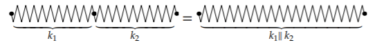
Exercise \(\PageIndex{4}\): Springs as capacitors

Using the analogy between springs and capacitors (discussed in Section 2.4.1), explain why springs in series combine using the parallel combination of their spring constants.

Another surprising example is the following spring–mass system with two masses:

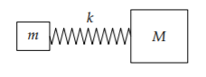
The natural frequency \(\omega\), expressed without our \(\parallel\) abstraction, is

\[\omega = \frac{k(m + M)}{mM}\]

This form looks complicated until we use the \(\parallel\) abstraction:

\[\omega = \frac{k}{m \parallel M}\]

Now the frequency makes more sense. The two masses act like their parallel combination \(m \parallel M\)

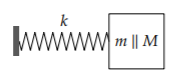
The replacement mass \(m \parallel M\) is so useful that it has a special name: the reduced mass. Our abstraction organizes complexity by turning a three-component system (a spring and two masses) into a simpler two-component system.

In the spirit of notation that promotes insight, use lowercase (“small”) m for the mass that is probably smaller, and uppercase (“big”) M for the mass that is probably larger. Then write \(m \parallel M\) rather than \(M \parallel m\). These two forms produce the same result, but the \(m \parallel M\) order minimizes surprise: The parallel combination of m and M is smaller than either mass (Problem 2.17), so it is closer to m, the smaller mass, than to M. Writing \(m \parallel M\), rather than \(M \parallel m\), places the most salient information first.

Exercise \(\PageIndex{5}\): Using the resistance analogy

By using the analogy with parallel resistances, explain why \(m \parallel M\) is smaller than m and M.

Why do the two masses combine like resistors in parallel?

The answer lies in the analogy between mass and resistance. Resistance appears in Ohm’s law:

voltage = resistance × current.

Voltage is an effort. Current, which results from the effort, is a flow. Therefore, the more general form—one step higher on the abstraction ladder—is

effort = resistance × flow.

In this form, Newton’s second law,

force = mass × acceleration

identifies force as the effort, mass as the resistance, and acceleration as the flow.

Because the spring can wiggle either mass, just as current can flow through either of two parallel resistors, the spring feels a resistance equal to the parallel combination of the resistances—namely, \(m \parallel M\).

Exercise \(\PageIndex{6}\): Three springs connected

What is the effective spring constant of three springs connected in a line, with spring constants 2, 3, and 6 newtons per meter, respectively?

2.4.4 Impedance as a higher-level abstraction

Resistance, in the electrical sense, has appeared several times, and it underlies a higher-level abstraction: impedance. Impedance extends the idea of electrical resistance to capacitors and inductors. Capacitors and inductors, along with resistors, are the three linear circuit elements: In these elements, the connection between current and voltage is described by a linear equation: Forresistors, it is a linear algebraic relation (Ohm’s law); for capacitors or inductors, it is a linear differential equation.

Why should we extend the idea of resistance?

Resistors are easy to handle. When a circuit contains only resistors, we can immediately and completely describe how it behaves. In particular, we can write the voltage at any point in the circuit as a linear combination of the voltages at the source nodes. If only we could do the same when the circuit contains capacitors and inductors.

We can! Start with Ohm’s law,

\[\textrm{current} = \frac{voltage}{resistance}\],

and look at it in the higher-level and expanded form

\[flow = \frac{1}{resistance} \times effort\]

For a capacitor, flow will still be current. But we’ll need to find the capacitive analog of effort. This analogy will turn out slightly different from the electrical–mechanical analogy between capacitance and spring constant (Section 2.4.1), because now we are making an analogy between capacitors and resistors (and, eventually, inductors). For a capacitor,

\[charge = capacitance \times voltage\]

To turn charge into current, we differentiate both sides to get

\[\textrm{current} = \textrm{capacitance} \times \frac{d\textrm{(voltage)}}{dt}\]

To make the analogy quantitative, let’s apply to the capacitor the simplest voltage whose form is not altered by differentiation:

\[V = V_{0}e^{j \omega t}\]

where V is the input voltage, V₀ is the amplitude, \(\omega\) is the angular frequency, and j is the imaginary unit \(\sqrt -1\). The voltage V is a complex number; but the implicit understanding is that the actual voltage is the real part of this complex number. By finding how the current I (the flow) depends on V (the effort), we will extend the idea of resistance to a capacitor.

With this exponential form, how can we represent the more familiar oscillating voltages V₁ cos \(\omega\)t or V₁ sin \(\omega\)t, where V₁ is a real voltage?

Start with Euler’s relation:

\[e^{j \omega t} = \cos \omega t + j \sin \omega t \]

To make V₁ cos \(\omega\) t, set \(V_{0} = V_{1}\) in \(V = V_{0} e^{j \omega t}\). Then

\[V= V_{1}(\cos \omega t + j \sin \omega t)\]

and the real part of V is just V₁ cos \(\omega\) t.

Making V₁ sin \(omega\) t is more tricky. Choosing \(V_{0} = j V_{1}\) almost works:

\[V= j V_{1} (\cos \omega t + j \sin \omega t) = V_{1} (j \cos \omega t - \sin \omega t)\].

The real part is \(-V_{1} \sin \omega t\), which is correct except for the minus sign. Thus, the correct amplitude is \(V_{0} = -jV_{1}\). In summary, our exponential form can compactly represent the more familiar sine and cosine signals.

With this exponential form, differentiation is simpler than with sines or cosines. Differentiating V with respect to time just brings down a factor of \(j \omega\), but otherwise leaves the \(V_{0} e^{j \omega t}\) alone:

\[\frac{dV}{dt} = j \omega \times V_{0} e^{j \omega t} = j \omega V\]

With this changing voltage, the capacitor equation,

\[current = capacitance \times \frac{d(voltage)}{dt}\]

becomes

\[current = capacitance \times j \omega \times voltage\]

Let's compare this form to its analog for a resistor (Ohm's law):

\[current = \frac{1}{resistance} \times voltage\]

Matching up the pieces, we find that a capacitor offers a resistance

\[Z_{C} = \frac{1}{j \omega C}\]

This more general resistance, which depends on the frequency, is called impedance and denoted Z. (In the analogy of Section 2.4.1 between capacitors and springs, we found that capacitor offered a resistance to being charged of 1/C. Impedance, the result of an analogy between capacitors and resistors, contains 1/C as well, but also contains the frequency in the 1/j \(\omega\) factor.)

Using impedance, we can describe what happens to any sinusoidal signal in a circuit containing capacitors. Our thinking is aided by the compact notation—the capacitive impedance ZC (or even RC). The notation hides the details of the capacitor differential equation and allows us to transfer our intuition about resistance and flow to a broader class of circuits.

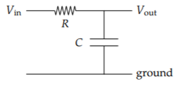
The simplest circuit with resistors and capacitors is the so-called low-pass RC circuit. Not only is it the simplest interesting circuit, it will also be, thanks to further analogies, a model for heat flow. Let's apply the impedance analogy to this circuit.

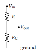
To help us make and use abstractions, let’s imagine defocusing our eyes. Under blurry vision, the capacitor looks like a resistor that just happens to have a funny resistance \(RC = \frac{1}{j \omega C}\). Now the entire circuit looks just like a pure-resistance circuit. Indeed, it is the simplest such circuit, a voltage divider. Its behavior is described by one number: the gain, which is the ratio of output to input voltage \(V_{out}/V_{in}\).

In the RC circuit, thought of as a voltage divider,

\[gain = \frac{\textrm{capacitive resistance}}{\textrm{total resistance from } V_{in} \textrm{to ground}} = \frac{R_{C}}{R+R_{C}}\]

Because \(R_{C} = \frac{1}{j \omega C}\), the gain becomes

\[gain = \frac{\frac{1}{j \omega C}}{R + \frac{1}{j \omega C}}\]

After clearing the fractions by multiplying by \(j \omega C\) in the numerator and denominator, the gain simplifies to

\[gain = \frac{1}{1 + j \omega R C}\]

Why is the circuit called a low-pass circuit?

At high frequencies (\(\omega\) → ∞), the \(j \omega R C\) term in the denominator makes the gain zero. At low frequencies (\(\omega\) → 0), the \(j \omega RC\) term disappears and the gain is 1. High-frequency signals are attenuated by the circuit; low-frequency signals pass through mostly unchanged. This abstract, high-level description of the circuit helps us understand the circuit without our getting buried in equations. Soon we will transfer our understanding of this circuit to thermal systems.

The gain contains the circuit parameters as the product RC. In the denominator of the gain, \(j \omega RC\) is added to 1; therefore, \(j \omega RC\), like 1, must have no dimensions. Because j is dimensionless (is a pure number), \(\omega RC\) must be itself dimensionless. Therefore, the product RC has dimensions of time. This product is the circuit’s time constant—usually denoted \(\tau\).

The time constant has two physical interpretations. To construct them, we imagine charging the capacitor using a constant input voltage V₀; eventually (after an infinite time), the capacitor charges up to the input voltage (V_out = V₀) and holds a charge \(Q=CV_{0}\). Then, at t= 0, we make the input voltage zero by connecting the input to ground.

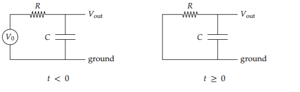
The capacitor discharges through the resistor, and its voltage decays exponentially:

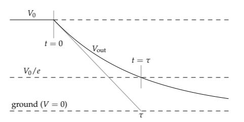
After one time constant \(\tau\), the capacitor voltage falls by a factor of e toward its final value—here, from V₀ to V₀/e. The 1/e time is our first interpretation of the time constant. Furthermore, if the capacitor voltage had decayed at its initial rate (just after t = 0), it would have reached zero voltage after one time constant \(\tau\)—the second interpretation of the time constant.

The time-constant abstraction hides—abstracts away—the details that produced it: here, electrical resistance and capacitance. Nonelectrical systems can also have a time constant but produce it by a different mechanism. Our high-level understanding of time constants, because it is not limited to electrical systems, will help us transfer our understanding of the electrical low-pass filter to nonelectrical systems. In particular, we are now ready to understand heat flow in thermal systems.

Exercise \(\PageIndex{7}\): Impedance of an inductor

An inductor has the voltage–current relation

\[V = L \frac{dI}{dt}\]

where L is the inductance. Find an inductor’s frequency-dependent impedance ZL. After finding this impedance, you can analyze any linear circuit as if it were composed only of resistors.

2.4.5 Thermal systems

The RC circuit is a model for thermal systems—which are not obviously connected to circuits. In a thermal system, temperature difference, the analog of voltage difference, produces a current of energy. Energy current, in less fancy words, is heat flow. Furthermore, the current is proportional to the temperature difference—just as electric current is proportional to voltage difference. In both systems, flow is proportional to effort. Therefore, heat flow can be understood by using circuit analogies.

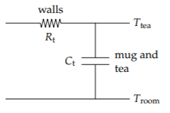
As an example, I often prepare a cup of tea but forget to drink it while it is hot. Like a discharging capacitor, the tea slowly cools toward room temperature and becomes undrinkable. Heat flows out through the mug. Its walls provide a thermal resistance; by analogy to an RC circuit, let's denote the thermal resistance R_t. The heat is stored in the water and mug, which form a heat reservoir. This reservoir, of heat rather than of charge, provides the thermal capacitance, which we denote C_t. (Thus the mug participates in the thermal resistance and capacitance.) Resistance and capacitance are transferable ideas.

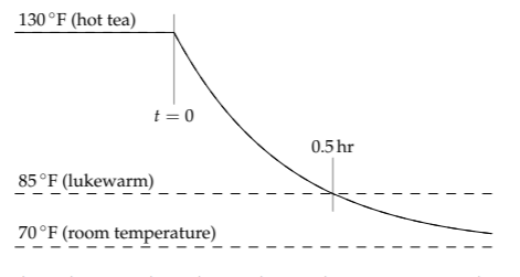
The product R_tC_t is, by analogy to the RC circuit, the thermal time constant \(\tau\). To estimate \(\tau\) with a home experiment (the method we used in Section 1.7), heat up a mug of tea; as it cools, sketch the temperature gap between the tea and room temperature. In my extensive experience of tea neglect, an enjoyably hot cup of tea becomes lukewarm in half an hour. To quantify these temperatures, enjoyably warm may be 130 °F (≈ 55 °C),room temperature is 70 °F (≈ 20 °C), and lukewarm may be 85 °F (≈ 30 °C).

Based on the preceding data, what is the approximate thermal time constant of the mug of tea?

In one thermal time constant, the temperature gap falls by a factor of e (just as the voltage gap falls by a factor of e in one electrical time constant). For my mug of tea, the temperature gap between the tea and the room started at 60 °F:

\[\underbrace{\textrm{enjoyably warm}}_{130^{o}F} - \underbrace{\textrm{room temperature}}_{70^{o}F} = 60^{o}F.\]

In the half hour while the tea cooled in the microwave, the temperature gap fell to 15°F:

\[\underbrace{\textrm{lukewarm}}_{85^{o}F} - \underbrace{\textrm{room temperature}}_{70^{o}F} = 15^{o}F.\]

Therefore, the temperature gap decreased by a factor of 4 in half an hour. Falling by the canonical factor of e (roughly 2.72) would require less time: perhaps 0.3 hours (roughly 20 minutes) instead of 0.5 hours. A more precise calculation would be to divide 0.5 hours by ln 4, which gives 0.36 hours. However, there is little point doing this part of the calculation so precisely when the input data are far less precise. Therefore, let’s estimate the thermal time constant \(\tau\) as roughly 0.3 hours.

Using this estimate, we can understand what happens to the tea mug when, as it often does, it spends a lonely few days in the microwave, subject to the daily variations in room temperature. This analysis will become our model for the daily temperature variations in a house.

How does a teacup with \(\tau\) ≈ 0.3 hours respond to daily temperature variations?

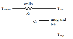
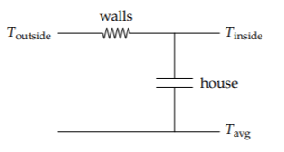
First, set up the circuit analogy. The output signal is still the tea's temperature. The input signal is the (sinusoidally) varying room temperature. However, the ground signal, which is our reference temperature, cannot also be the room temperature. Instead, we need a constant reference temperature. The simplest choice is the average room temperature T_avg. (After we have transferred this analysis to the temperature variation in houses, we'll see that the conclusion is the same even with a different reference temperature.)

The gain connects the amplitudes of the output and input signals:

\[gain = \frac{\textrm{amplitude of the output signal}}{\textrm{amplitude of the input signal}} = \frac{1}{1 + j \omega \tau}\]

The input signal (room temperature) varies with a frequency f of 1 cycle per day. Then the dimensionless parameter \(\omega \tau\) in the gain is roughly 0.1. Here is that calculation:

\[\underbrace{2 \pi \times \overbrace{1 \frac{\textrm{cycle}}{\textrm{day}}}^{f}}_{\omega} \times \underbrace{0.3 \textrm{ hr}}_{\tau} \times \underbrace{\frac{1 \textrm{day}}{24 \textrm{hr}}}_{1} \approx 0.1.\]

The system is driven by a low-frequency signal: \(\omega\) is not large enough to make \(\omega \tau\) comparable to 1. As the gain expression reminds us, the mug of tea is a low-pass filter for temperature variations. It transmits this low-frequency input temperature signal almost unchanged to the output—to the tea temperature. Therefore, the inside (tea) temperature almost exactly follows the outside (room) temperature.

The opposite extreme is a house. Compared to the mug, a house has a much higher mass and therefore thermal capacitance. The resulting time constant \(\tau = R_{t}C_{t}\) is probably much longer for a house than for the mug. As an example, when I taught in sunny Cape Town, where houses are often unheated even in winter, the mildly insulated house where I stayed had a thermal time constant of approximately 0.5 days.

For this house the dimensionless parameter \(\omega \tau\) is much larger than it was for the tea mug. Here is the corresponding calculation.

\[\underbrace{2 \pi \times \overbrace{1 \frac{\textrm{cycle}}{\textrm{day}}}^{f}}_{\omega} \times \underbrace{0.5 \textrm{days}}_{\tau} \approx 3.\]

What consequence does \(\omega \tau \approx 3\) have for the indoor temperature? In the Cape Town winter, the outside temperature varied daily between 45 °F and 75 °F; let’s also assume that it varied approximately sinusoidally. This 30 °F peak-to-peak variation, after passing through the house low-pass filter, shrinks by a factor of approximately 3. Here is how to find that factor by estimating the magnitude of the gain.

\[|gain| = |\frac{\textrm{amplitude of }T_{inside}}{\textrm{amplitude of } T_{outside}}| = |\frac{1}{1 + j \omega \tau}|\]

(It is slightly confusing that the outside temperature is the input signal, and the inside temperature is the output signal!) Now plug in \(\omega \tau \approx 3\) to get

\[|gain| \approx |\frac{1}{1 + 3j}| = \frac{1}{\sqrt{1^{2} + 3^{2}}} \approx \frac{1}{3}\]

In general, when \(\omega \tau\) ≫ 1, the magnitude of the gain is approximately 1/\(\omega \tau\).

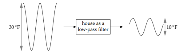
Therefore, the outside peak-to-peak variation of 30 °F becomes a smaller inside peak-to-peak variation of 10 °F. Here is a block diagram showing this effect of the house low-pass filter.

Our comfort depends not only on the temperature variation (I like a fairly steady temperature), but also on the average temperature.

What is the average temperature indoors?

It turns out that the average temperature indoors is equal to the average temperature outdoors! To see why, let’s think carefully about the reference temperature (our thermal analog of ground). Before, in the analysis of the forgotten tea mug, our reference temperature was the average indoor temperature. Because we are now trying to determine this value, let’s instead use a known convenient reference temperature—for example, the cool 10 °C, which makes for round numbers in Celsius or Fahrenheit (50 °F).

The input signal (the outside temperature) varied in winter between 45° F and 75°F. Therefore, it has two pieces: (1) our usual varying signal with the 30°F peak-to-peak variation, and (2) a steady signal of 10°F.

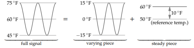
The steady signal is the difference between the average outside temperature of 60°F and the reference signal of 50°F.

Let’s handle each piece in turn—we are using divide-and-conquer reasoning again. We just analyzed the varying piece: It passes through the house low-pass filter and, with \(\omega \tau \approx 3\), it shrinks significantly in amplitude. In contrast, the nonvarying part, which is the average outside temperature, has zero frequency by definition. Therefore, its dimensionless parameter \(\omega \tau\) is exactly 0. This signal passes through the house low-pass filter with a gain of 1. As a result, the average output signal (the inside temperature) is also 60°F: the same steady 10°F signal measured relative to the reference temperature of 50°F.

The 10°F peak-to-peak inside-temperature amplitude is a variation around 60°F. Therefore, the inside temperature varies between 55°F and 65°F (13°C to 18°C). Indoors, when I am not often running or otherwise generating much heat, I feel comfortable at 68°F (20°C). So, as this circuit model of heat flow predicts, I wore a sweater day and night in the Cape Town house. (For more on using RC circuit analogies for building design, see the “Design masterclass” article by Doug King [30].)

Exercise \(\PageIndex{8}\): When is the house coldest?

Based on the general form for the gain, \(1/(1 + j \omega \tau\)), when in the day will the Cape Town house be the coldest, assuming that the outside is coldest at midnight?