3.4: Box Models and Conservation

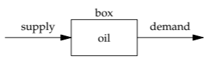
Invariance underlies a powerful everyday abstraction: box models. We already made a box model in Section 3.1.1, to decide whether to run or walk in the rain. Now let’s examine this method further. The simplest kind of box contains a fixed amount of stuff—perhaps the volume of fluid or the number of students at an ideal university (where every student graduates in a fixed time). Then what goes into the box must come out. This conclusion seems simple, even simplistic, but it has wide application.

3.4.1 Supply and demand

For another example of a box model,return to our estimate of US oil usage (Section 1.4). The flow into the box—the push or the supply—is the imported and domestically produced oil. The flow out of the box—the pull or the demand—is the oil usage. The estimate, literally taken, asks for the supply (how much oil is imported and domestically produced). This estimate is difficult. Fortunately, as long as oil does not accumulate in the box (for example, as long as oil is not salted away in underground storage bunkers), then the amount of oil in the box is an invariant, so the supply equals the demand. To estimate the supply, we accordingly estimated the demand. This conservation reasoning is the basis of the following estimate of a market size.

How many taxis are there in Boston, Massachusetts?

For many car-free years, I lived in an old neighborhood of Boston. I often rode in taxis and wondered about the size of the taxi market—in particular, how many taxis there were. This number seemed hard to estimate, because taxis are scattered throughout the city and hard to count.

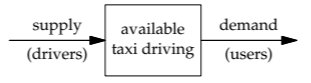
The box contains the available taxi driving (measured, for example, as time). It is supplied by taxi drivers. The demand is due to taxi users. As long as the supply and demand match, we can estimate the supply by estimating the demand

For estimating the demand, the starting point is that Boston has roughly 500 000 residents. As a gut estimate, each resident uses maybe one taxi per month, for a 15-minute ride: Boston taxis are expensive; unless one doesn’t own a car, it’s hard to imagine using them more often than once a month or for longer than 15 minutes. Then the demand is about 105 hours of taxi driving per month:

\[5 \times 10^{5} \cancel{residents} \times \frac{15 \cancel{min}}{\cancel{resident} month} \times \frac{1hr}{60 \cancel{min}} \approx \frac{10^{5} hr}{month}.\]

How many taxi drivers will that many monthly hours support?

Taxi drivers work long shifts, maybe 60 hours per week. I’d guess that they carry passengers one-half of that time: 30 hours per week or roughly 100 hours per month. At that pace, 10⁵ hours of monthly demand could be supplied by 1000 taxi drivers or, assuming each taxi is driven by one driver, by 1000 taxis.

What about tourists?

Tourists are very short-term Boston residents, mostly without cars. Tourists, although fewer than residents, use taxis more often and for longer than residents do. To include the tourist contribution to taxi demand, I’ll simply double the previous estimate to get 2000 taxis.

This estimate can be checked reliably, because Boston is one of the United States cities where taxis may pick up passengers only with a special permit, the medallion. The number of medallions is strictly controlled, so medallions cost a fortune. For about 60 years, their number was restricted to 1525, until a 10-year court battle got the limit raised by 260, to about 1800.

The estimate of 2000 may seem more accurate than it deserves. However, chance favors the prepared mind. We prepared by using good tools: a box model and divide-and-conquer reasoning. In making your own estimates, have confidence in the tools, and expect your estimates to be at least half decent. You will thereby find the courage to start: Optimism oils the rails of estimation

Exercise \(\PageIndex{1}\): Differential equation for an RC circuit

Explain how a box model leads to the differential equation for the low-pass RC circuit of Section 2.4.4:

\[RC\frac{dV_{out}}{dt} + V_{out} = V_{in}.\]

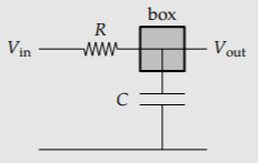
(Almost every differential equation arises from a box or conservation argument.)

Exercise \(\PageIndex{2}\): Boston taxicabs tree

Draw a divide-and-conquer tree for estimating the number of Boston taxicabs. First draw it without estimates. Then include your estimates, and propagate the values toward the root.

Exercise \(\PageIndex{3}\): Needles on a Christmas tree

Estimate the number of needles on a Christmas tree

3.4.2 Flux

Flows, such as the demand for oil or the supply of taxi cabs, are rates—an amount per time. Physical flows are also rates, but they live in a geometry. This embedding allows us to define a related quantity: flux.

\[\textrm{flux of stuff} \equiv \frac{rate}{area} = \frac{\textrm{amount of stuff}}{area \times time}\]

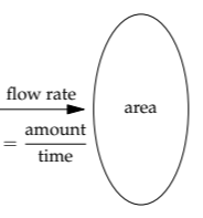
For example, particle flux is the rate at which particles (say, molecules) pass through a surface perpendicular to the flow, divided by the area of the surface. Dividing by the surface area, an operation with no counterpart in nonphysical flows (for example, in the demand for taxicabs), makes flux more invariant and useful than rate. For if you double the surface area, you double the rate. This proportionality is not newsworthy, and usually doesn’t add insight, only clutter. When there is change, look for what does not change: Even when the area changes, flux does not.

Exercise \(\PageIndex{4}\): Rate versus amount

Explain why rate (amount per time) is more useful than amount.

Exercise \(\PageIndex{5}\): What is current density

What kind of flux (flux of what?) is current density (current per area)?

The definition of flux leads to a simple and important connection between flux and flow speed. Imagine a tube of stuff (for example, molecules) with cross-sectional area A. The stuff flows through the tube at a speed v.

In a time t, how much stuff leaves the tube?

In the time t, the stuff in the shaded chunk, spanning a length vt, leaves the tube. This chunk has volume Avt. The amount of stuff in that volume is

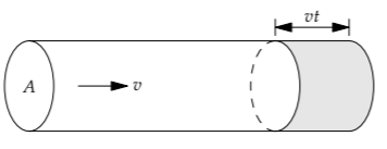
\[\underbrace{\frac{\textrm{stuff}}{\textrm{volume}}}_{\textrm{density of stuff}} \times \underbrace{Avt}_{\textrm{volume}}.\]

The amount of stuff per volume, the density of stuff, occurs so often that it usually gets a special symbol. When the stuff is particles, the density is labeled n for number density (in contrast to N for the number itself). When the stuff is charge or mass, the density is labeled \(\rho\).

From the amount of stuff, we can find the flux:

\[\textrm{flux of stuff} = \frac{\textrm{amount of stuff}}{\textrm{area} \times \textrm{time}} = \frac{\textrm{density of stuff} \times \overbrace{\textrm{volume}}^{Avt}}{\underbrace{\textrm{area} \times \textrm{time}}_{At}}.\]

The product At cancels, leaving the general relation

\[\textrm{flux of stuff} = \textrm{density of stuff} \times \textrm{flow speed}\]

As a particular example, when the stuff is charge (Problem 3.28), the flux of stuff becomes charge per time per area, which is current per area or current density. With that label for the flux, the general relation becomes

\[\underbrace{\textrm{current density}}_{J} = \underbrace{\textrm{charge density}}_{\rho} \times \underbrace{\textrm{flow speed}}_{v_{drift}},\]

where v_drift is the flow speed of the charge—which you will estimate in Problem 6.16 for electrons in a wire.

The general relation will be crucial in estimating the power required to fly (Section 3.6) and in understanding heat conduction (Section 7.4.2).

3.4.3 Average solar flux

An important flux is energy flux: the rate at which energy passes through a surface, divided by the area of the surface. Here, rate means energy per time, or power. Therefore, energy flux is power per area. An energy flux essential to life is the solar flux: the solar power per area falling on Earth. This flux drives most of our weather. At the top of the atmosphere, looking directly toward the sun, the flux is roughly F = 1300 watts per square meter.

However, this flux is not evenly distributed over the surface of the earth. The simplest reason is night and day. On the night side of the Earth, the solar flux is zero. More subtly, different latitudes have different solar fluxes: The equatorial regions are warmer than the poles because they receive more solar flux than the poles do.

What is the solar flux averaged over the whole Earth?

We can find the average flux using a box model (a conservation argument). Here is sunlight coming to the Earth (with parallel rays, because the Sun is so far away). Hold a disk with radius R_Earth perpendicular to the sunlight so that it blocks all sunlight that the Earth otherwise would get. The disk absorbs a power that we can find from the energy flux:

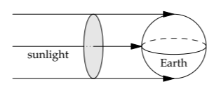
\[power = energy \: flux \times area = F \pi R^{2}_{Earth},\]

where F is the solar flux. Now spread this power over the whole Earth, which has surface area \(4 \pi R^{2}_{Earth}\):

\[\textrm{average flux} = \frac{power}{\textrm{surface area}} = \frac{F \pi R^{2}_{Earth}}{4 \pi R^{2}_{Earth}} = \frac{F}{4}\]

Because one-half of the Earth is in night, averaging over the night and daylight parts of the earth accounts for a factor of 2. Therefore, averaging over latitudes must account for another factor of 2 (Problem \(\PageIndex{6}\)).

Exercise \(\PageIndex{6}\): Averaging solar flux over all latitudes

Integrate the solar flux over the whole sunny side of the Earth, accounting for the varying angles between the incident sunlight and the surface. Check that the result agrees with the result of the box model.

The result is roughly 325 watts per square meter. This average flux slightly overestimates what the Earth receives at ground level, because not all of the 1300 watts per square meter hitting the top of the atmosphere reaches the surface. Roughly 30 percent gets reflected near the top of the atmosphere (by clouds). The surviving amount is about 1000 watts per square meter. Averaged over the surface of the Earth, it becomes 250 watts per square meter(which then goes into the surface and the atmosphere), or approximately F/5, where F is the flux at the top of the atmosphere.

3.4.4 Rainfall

These 250 watts per square meter determine characteristics of our weather that are essential to life: the average surface temperature and the average rainfall. You get to estimate the surface temperature in Problem 5.43, once you learn the reasoning tool of dimensional analysis. Here, we will estimate the average rainfall.

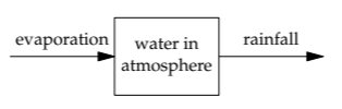
If the box representing the atmosphere holds a fixed amount of water—and over a long timescale, the amount is constant (it is our invariant)—then what goes into the box must come out of the box. The inflow is evaporation; the outflow is rain. Therefore, to estimate the rainfall, estimate the evaporation—which is produced by the solar flux.

How much rain falls on Earth?

Rainfall is measured as a height of water per time—typically, inches or millimeters per year. To estimate global average rainfall, convert the supply of solar energy to the supply of rainwater. In other words, convert power per area to height per time. The structure of the conversion is

\[\frac{power}{area} \times {?}{?} = \frac{height}{time},\]

where ?/? represents the conversion factor that we need to determine. To find what this conversion factor represents, we multiply both sides by area per power. The result is

\[\frac{?}{?} = \frac{area \times height}{power \times time} = \frac{volume}{energy}.\]

What physical quantity could this volume per energy be?

We are trying to determine the amount of rain, so the volume in the numerator must be the volume of rain. Evaporating the water requires energy in the denominator must be the energy required to evaporate that much water. The conversion factor is then the reciprocal of the heat of vaporization of water L_vap, but expressed as an energy per volume. In Section 1.7.3, we estimated L_vap as an energy per mass. To make it an energy per volume, just multiply by a mass per volume--namely, by \(\rho_{water}\).

\[\underbrace{\frac{\textrm{energy}}{\cancel{\textrm{mass}}}}_{L_{vap}} \times \underbrace{\frac{\cancel{\textrm{mass}}}{\textrm{volume}}}_{\rho_{water}} = \underbrace{\frac{\textrm{energy}}{\textrm{volume}}}_{\rho_{water}L_{vap}}}.\]

Our conversion factor, volume per energy, is the reciprocal, \[\frac{1}{\rho_{water} L_{vap}\]. Our estimate for the average rainfall then becomes

\[\frac{\textrm{solar flux going to evaporate water}}{\rho_{water}L_{vap}}\]

For the numerator, we cannot just use F, the full solar flux at the top of the atmosphere. Rather, the numerator incorporates several dimensionless ratios that account for the hoops through which sunlight must jump in order to reach the surface and evaporate water.

0.25 averaging the intercepted flux over the whole surface of the Earth (Section 3.4.3)

0.7 the fraction not reflected at the top of the atmosphere

0.7 of the sunlight not reflected, the fraction reaching the surface (the other 30 percent is absorbed in the atmosphere)

× 0.7 of the sunlight reaching the surface, the fraction reaching the oceans (the other 30 percent mostly warms land)

= 0.09 fraction of full flux F that evaporates water (including averaging the full flux over the whole surface)

The product of these four factors is roughly 9 percent. With L_vap = 2.2 × 10⁶ joules per kilogram (which we estimated in Section 1.7.3), our rainfall estimate becomes roughly

\[\frac{\overbrace{1300 \textrm{W m}^{-2}}^{F} \times \overbrace{0.09}^{\textrm{fraction}}}{\underbrace{10^{3} \textrm{kg m}^{-3}}_{\rho_{water}} \times \underbrace{2.2 \times 10^{6} \textrm{J kg}^{-3}}_{L_{vap}}} \approx \frac{5.3 \times 10^{-8} m}{s}.\]

The length in the numerator is tiny and hard to perceive. Therefore, the common time unit for rainfall is a year rather than a second. To convert the rainfall estimate to meters per year, multiply by 1:

\[\frac{5.3 \times 10^{-8} m}{\cancel{s}} \times \frac{3 \times 10^{7} \cancel{s}}{1 yr} \approx \frac{1.6m}{yr}\]

(about 64 inches per year). Not bad: Including all forms of falling water, such as snow, the world average is 0.99 meters per year—slightly higher over the oceans and slightly lower over land (where it is 0.72 meters per year). The moderate discrepancy between our estimate and the actual average arises because some sunlight warms water without evaporating it. To reflect this effect, our table on page 81 needs one more fraction (≈ 2/3).

Exercise \(\PageIndex{7}\):Solar luminosity

Estimate the solar luminosity—the power output of the Sun (say, in watts)—based on the solar flux at the top of the Earth’s atmosphere.

Exercise \(\PageIndex{8}\): Total solar power falling on Earth

Estimate the total solar power falling on the Earth’s surface. How does it compare to the world energy consumption?

Exercise \(\PageIndex{9}\): Explaining the difference between ocean and land rainfall

Why is the average rainfall over land lower than over the ocean?

3.4.5 Residence times

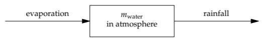
Because of evaporation, the atmosphere contains a lot of water: roughly 1.3×10¹⁶ kilograms—as vapor, liquid, and solid. This mass tells us the residence time: how long a water molecule remains in the atmosphere before it falls back to the Earth as precipitation (the overall name for rain, snow, or hail). The estimate will illustrate a new way to use box models.

Here is the box representing the water in the atmosphere (assumed to need only one box). The box is filled by evaporation and emptied by rainfall.

Imagine that the box is a water hose holding a mass m_water. How long does a water molecule take to get from one end of the hose to other? This time is the average time taken by a water molecule from evaporation until its return to the Earth as precipitation. In the box model, the time is the time to completely fill the box. This time constant, denoted \(\tau\), is

\[\tau = \frac{\textrm{mass of water in the atmosphere}}{\textrm{rate of inflow or outflow, as a mass per time}.\]

The numerator is m_water. For the denominator, we convert rainfall, which is a speed (for example, in meters per year), to a mass flow rate (mass per time). Let's name the rainfall speed v_rainfall. The corresponding mass flux is, using our results from Section 3.4.2, \(\rho_{water}v_{rainfall}\):

\[\textrm{mass flux} = \underbrace{\textrm{density}}_{\rho_{water}} \times \underbrace{\textrm{flow speed}}_{v_{rainfall}} = \rho_{water}v_{rainfall}.\]

Flux is flow per area, so we multiply mass flux by the Earth’s surface area A_Earth to get the mass flow:

\[\textrm{mass flow} = \rho_{water}v_{rainfall}A_{Earth}.\]

At this rate, the fill time is

\[\tau = \frac{m_{water}}{\rho_{water}v_{rainfall}A_{Earth}}.\]

There are two ways to evaluate this time: the direct but less insightful method, and the less direct but more insightful method. Let’s first do the direct method, so that we at least have an estimate for \(\tau\).

\[\tau \sim \frac{1.3 \times 10^{16}kg}{10^{3}kg m^{-3} \times 1 m yr^{-1} \times 4 \pi \times (6 \times 10^{6}m)^{2}} \approx 2.5 \times 10^{-2} yr,\]

which is roughly 10 days. Therefore, after evaporating, water remains in the atmosphere for roughly 10 days.

For the less direct but more insightful method, notice which quantities are not reasonably sized—that is, not graspable by our minds—namely, m_water and A_Earth. But the combination \(m_{water}/\rho_{water}A_{Earth}\) is reasonably sized:

\[\frac{m_{water}}{\rho_{water}A_{Earth}} \sim \frac{1.3 \times 10^{16} kg}{10^{3}kg m^{-3} \times 4 \pi \times (6 \times 10^{6} m)^{2}} \approx 2.5 \times 10^{-2} m.\]

This length, 2.5 centimeters, has a physical interpretation. If all water, snow, and vapor fell out of the atmosphere to the surface of the Earth, it would form an additional global ocean 2.5 centimeters deep.

Rainfall takes away 100 centimeters per year. Therefore, draining this ocean, with a 2.5-centimeter depth, requires 2.5×10⁻² years or about 10 days. This time is, once again, the residence time of water in the atmosphere.