
5.4: Temperature and change
- Page ID
- 24110

The preceding examples of dimensional analysis have been mechanical, using the dimensions of length, mass, and time. Temperature and charge are also essential to describing the world and are equally amenable to dimensional analysis. Let’s start with temperature.
5.4.1 Temperature
To handle temperature, do we need to add another fundamental dimension?
Representing temperature as a new fundamental dimension is one method, and the dimension is symbolized by \(\Theta\). However, there’s a simpler method. It uses another fundamental constant of nature: Boltzmann’s constant kB. It has dimensions of energy per temperature; thus, it connects temperature to energy. In SI units, kB is roughly 1.6 × 10⁻²³ joules per kelvin. When a temperature T appears, convert it to the corresponding energy kBT (just as we convert G, in gravity problems, to Gm).
For our first temperature example, let’s estimate the speed of air molecules. We will then use that knowledge to estimate the speed of sound. Because the speed \(v\) of air molecules is a result of thermal energy, it depends on kBT. But \(v\) and kBT—two quantities made from two independent dimensions—cannot make a dimensionless group. We need one more quantity: the mass m of an air molecule.
Although these three quantities contain three dimensions, only two of the dimensions are independent—for example, M and LT−1. Therefore, the three quantities produce one independent dimensionless group. A reasonable choice for it is \(mv^{2}/k_{B}T\). Then
| \(v\) | LT-1 | thermal speed |
| \(k_{B}T\) | ML2T-2 | thermal energy |
| \(m\) | M | molecular mass |
This result is quite accurate. The missing dimensionless prefactor is \(\sqrt{3}\) for the root-mean-square speed and \(\sqrt{8/\pi}\) for the mean speed.
The dimensional-analysis result helps predict the speed of sound. In a gas, sound travels because of pressure, which is a result of thermal motion. Thus, it is plausible that the speed of sound cs should be comparable to the thermal speed. Then,
\[c_{s} \sim \sqrt{\frac{k_{B}T}{m}}.\]
To evaluate the speed numerically, multiply by a form of 1 based on Avogadro’s number:
\[c_{s} \sim \sqrt{\frac{k_{B}T}{m} \times \frac{N_{A}}{N_{A}}}.\]
The numerator now contains \(k_{B}N_{A}\), which is the universal gas constant R:
\[R \approx \frac{8J}{mol K}.\]
The denominator in the square root is \(mN_{A}\): the mass of one molecule multiplied by Avogadro's number. It is therefore the mass of one mole of air molecules. Air is mostly N2, with an atomic mass of 28. Including the oxygen for us animals, the molar mass of air is roughly 30 grams per mole. Plugging in 300K for room temperature gives a thermal speed of roughly 300 meters per second:
\[c_{s} \sim \sqrt{\frac{8J mol^{-1}K^{-1} \times 300K}{3 \times 10^{-2}kg mol^{-1}}} \approx 300 m s^{-1}.\]
The actual sound speed is 340 meters per second, not far from our estimate based on dimensional analysis and a bit of physical reasoning. (The discrepancy remaining is due to the difference between isothermal and adiabatic compression and expansion. For a related effect, later try Problem 8.27.)
With this understanding of how to handle temperature, let’s use dimensional analysis to estimate the height of the atmosphere. This height, called the scale height H, is the length over which the atmosphere’s properties, such as pressure and density, change significantly. At the height H, the atmospheric density and pressure will be significantly lower than at sea level.
The first step in dimensional analysis is to list the quantities that determine the height. That list requires a physical model: THe atmosphere is a competition between gravity and thermal motion. Gravity drags molecules toward Earth; thermal motion spreads them all over the universe. Our list must include quantities representing both sides of that competition: m and g for gravity, and \(k_{B}T\) for thermal energy.
| H | L | atmosphere height |
| g | LT-2 | gravity |
| \(k_{B}T\) | ML-2T-2 | thermal energy |
| m | M | molecular mass |
Four quantities (including the goal H) built from three independent dimensions produce one independent dimensionless group. A reasonable choice for the group—reasonable because it is proportional to the goal H—is the ratio \(mgH/k_{B}T\). Therefore, the atmosphere’s scale height is given by
\[H \sim \frac{k_{B}T}{mg}\]
To evaluate this height numerically, again convert Boltzmann’s constant kB to the universal gas constant R by multiplying by \(N_{A}/N_{A}\):
\[H \sim \frac{\overbrace{k_{B}N_{A}}^{R}T}{\underbrace{mN_{A}}_{m_{molar}}g} \approx \frac{\overbrace{8 \textrm{J mol}^{-1} \textrm{K}^{-1}}^{R} \times 300K}{\underbrace{3 \times 10^{-2} \textrm{ kg mol}^{-1}}_{m_{molar}} \times 10 \textrm{ m s}^{-2}} \approx 8 \textrm{ km.}\]
Thus, by 8 kilometers above sea level, atmospheric pressure and density should be significantly lower than at sea level. This conclusion is reasonable: Mount Everest is 9 kilometers high, where the significantly thinner air requires climbers to carry oxygen tanks.
As a rule of thumb for a decaying function such as atmospheric pressure or density, a “significant change” can be estimated as a rise or, here, a fall by a factor of \(e\) (For more on this rule of thumb, try Problem 6.36 after you have studied lumping; see also Section 3.2.1 of Street-Fighting Mathematics [33].) Indeed, at 8 kilometers, the standardized atmospheric parameters relative to sea level are \(\rho/\rho_{0} \approx 0.43\) and \(p/p_{0} \approx 0.35\). For comparison, \(1/e\) is approximately 0.37.
5.4.2 Charge
Our second new dimension is charge, symbolized by Q. By introducing charge, we can apply dimensional analysis to electrical phenomena. Let’s begin by finding the dimensions of electrical quantities
What are the dimensions of current, voltage, and resistance?
Current is the flow of charge; it has dimensions of charge per time. Using I to denote current and [I] to denote its dimensions
\[[I] = QT^{-1}\]
The dimensions of voltage can be determined from the relation
\[\textrm{voltage} \times \textrm{current} = \textrm{power}\]
The corresponding dimensional equation is
\[[voltage] = \frac{[power]}{[current]}.\]
Because the dimensions of power (energy per time) are ML2T-3, and the dimensions of current are QT-1, the dimensions of voltage are ML2T-2Q-1:
\[[voltage]= \frac{ML^{2}T^{-3}}{QT^{-1}} = ML^{2}T^{-2}Q^{-1}.\]
In this expression, the dimensional combination ML2T−2 is energy. Therefore, voltage is also energy per charge. As a result, an electron volt (1 electron charge times 1 volt) is an energy. A few electron volts is the energy in chemical bonds. Because chemical bonds reflect a change in one or two electrons, atomic and molecular voltages must be a few volts. (An everyday consequence is that typical batteries supply a few volts.)
To find the dimensions of resistance, we’ll write Ohm’s law as a dimensional equation:
\[[resistance] = \frac{[voltage]}{[current]} = \frac{ML^{2}T^{-2}Q^{-1}}{QT^{-1}} = ML^{2}T^{-1}Q^{-2}.\]
To simplify these dimensions, use [V]—the dimensions of voltage—as an abstraction for the dimensional mess ML2T−2Q−1. Then,
\[[resistance] = [V] \times TQ^{-1}.\]
This alternative is useful when the input to and output of a circuit is voltage. Then treating the dimensions of voltage as a fundamental dimension simplifies the task of finding dimensionless groups. (For practice in using the dimensions of voltage, try Problem \(\PageIndex{1}\).)
Exercise \(\PageIndex{1}\): Capacitance and inductance
Express the dimensions of capacitance and inductance using L, M, T, and Q. Then write them using [V] (the dimensions of voltage) along with any fundamental dimensions that you need.
Exercise \(\PageIndex{2}\): RC circuit
In this problem, you apply dimensional analysis to the low-pass RC circuit that we introduced in Section 2.4.4. In particular, make the input voltage Vin zero for time t < 0 and a fixed voltage V0 for t ≥ 0. The goal is the most general dimensionless statement about the output voltage V, which depends on V0, t, R, and C.
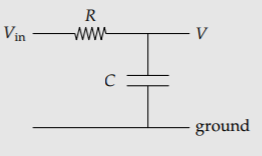
a. Using [V] to represent the dimensions of voltage, fill in a dimensional-analysis table for the quantities V, V0, t, R, and C.
b. How many independent dimensions are contained in these five quantities?
c. Form independent dimensionless groups and write the most general statement in the form
\[\textrm{group containing } V \textrm{ but not } t = f \textrm{(group containing } t \textrm{ but not } V, \textrm{ ...)}, \]
where the ... stands for the third dimensionless group (if it exists). Compare your expression to the analysis of the RC circuit in Section 2.4.4.
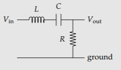
Exercise \(\PageIndex{3}\): Dimensional analysis of an LRC circuit
In the LRC circuit, the input voltage Vin is the real part of a complex-exponential signal \(V_{0}e^{j \omega t}\), where V0 is the input amplitude and \(\omega\) is the angular oscillation frequency. The output voltage Vout is then the real part of \(V_{1}e^{j \omega t}\), where V1 is the (possibly complex) output amplitude. What quantities determine the gain G, defined as the ratio V1/V0? What is a good set of independent dimensionless groups built from G and these quantities?
Along with the potential (or voltage) V, a leading actor in electromagnetics is the electric field. (Once you understand how to handle electric fields, you can practice by analyzing magnetic fields—try Problems 5.31, 5.32, and 5.33.) Electric fields not only transmit force; they also contain energy. This energy is important, not least because its transport is how the Sun warms the Earth. We will estimate the energy contained in electric fields by using dimensional analysis. This analysis will give us the result that we used in Section 2.4.2 to estimate, by analogy, the energy in a gravitational field. Like the gravitational field, the electric field extends over space. Therefore, we usually want not the energy itself, but rather the energy per volume—the energy density.
What is the energy density in an electric field?
To answer this question with dimensional analysis, let’s follow most of the steps that we used in estimating the bending of starlight (Section 5.3.1).
1. List the relevant quantities.
2. Form independent dimensionless groups.
3. Use the groups to make the most general statement about the energy density.
4. Narrow the possibilities by incorporating physical knowledge. For this problem, we will be able to skip this step.
Thus, the first step is to tabulate the quantities on which our goal, the energy density \(\varepsilon\), depends. It definitely depends on the electric field E. It also probably depends on \(\epsilon_{0}\), the permittivity of free space appearing in Coulomb’s law, because most results in electrostatics contain \(\epsilon_{0}\). But \(\varepsilon\) shouldn’t depend on the speed of light: The speed of light suggests radiation, which requires a changing electric field; however, even a constant electric field contains energy. Thus, our list might be complete. Let’s see, by trying to make a dimensionless group.
So we list the quantities with their dimensions, with the goal at the head of the table. Energy density is energy per volume, so its dimensions are ML−1T−2. Electric field is force per charge (just as gravitational field is force per mass—analogy!), so its dimensions are MLT−2Q−1.
| \(\varepsilon\) | ML-1T-2 | energy density |
| E | MLT-2Q-1 | electric field |
| \(epsilon_{0}\) | M-1L-3T2Q2 | SI constant |
What are the dimensions of \(\epsilon_{0}\)?
This quantity is the trickiest. It shows up in Coulomb’s law:
\[\textrm{electrostatic force} = \frac{q^{2}}{4 \pi \epsilon_{0}}\frac{1}{r^{2}}.\]
As a dimensional equation,
\[[\epsilon_{0}] = \frac{Q^{2}}{[F]L^{2}},\]
where [F] = MLT−2 represents the dimensions of force. Therefore, \(\epsilon_{0}\) has dimensions of M−1L−3T2Q2 .
The second step is to find independent dimensionless groups. Any search is aided by knowing how many items to find. This count is provided by the Buckingham Pi theorem. To apply the theorem, we first need to count the independent dimensions.
How many independent dimensions do the three quantities contain?
At first glance, the quantities contain four independent dimensions: M, L, T, and Q. However, the Buckingham Pi theorem would then predict −1 dimensionless groups, which is nonsense. Indeed, the number of independent dimensions cannot exceed the number of quantities (a restriction that you explained in Problem 5.7). Here, as you verify in Problem \(\PageIndex{4}\), there are only two independent dimensions—for example, MLT−2Q−1 (the dimensions of electric field) and L2Q−1.
Three quantities constructed from two independent dimensions produce one independent dimensionless group. A useful choice for this group, because it is proportional to the goal \(\varepsilon\), is \(\varepsilon/\epsilon_{0}E^{2}\).
The third step is to use the independent dimensionless group to make the most general statement about the energy density. With only one group, the most general statement is
\[\varepsilon \sim \epsilon_{0}E^{2}.\]
The fourth step is to narrow the possibilities by using physical knowledge. With only one independent dimensionless group, the space of possibilities is already narrow. The only freedom is the dimensionless prefactor hidden in the single approximation sign ~; it turns out to be 1/2. In Section 5.4.3, the scaling \(\varepsilon \: \alpha \: E^{2}\) will help us explain the surprising behavior of the electric field produced by an accelerating charge—and thereby explain why stars are visible and radios work.
Exercise \(\PageIndex{4}\): Rewriting the dimensions
Express the dimensions of \(\varepsilon\), E, and \(\epsilon_{0}\) in terms of [E] (the dimensions of electric field) and L2Q−1. Thus, show that the three quantities contain only two independent dimensions.
Exercise \(\PageIndex{5}\): Dimensions of magnetic field
A magnetic field B produces a force on a moving charge q given by
\[\textbf{F} = q(\textbf{v} \times \textbf{B}),\]
where v is the charge’s velocity. Use this relation to find the dimensions of magnetic field in terms of M, L, T, and Q. Therefore, give the definition of a tesla, the SI unit of magnetic field.
Exercise \(\PageIndex{6}\): Magnetic energy density
Just as electric fields depend on \(\epsilon_{0}\), the permittivity of free space, magnetic fields depend on the constant \(\mu_{0}\) called the permeability of free space. It is defined as
\[\mu_{0} \equiv 4 \pi \times 10^{-7} N A^{-2},\]
where N is a newton and A is an ampere (a coulomb per second). Express the dimensions of \(\mu_{0}\) in terms of M, L, T, and Q. Then use the dimensions of magnetic field (Problem \(\PageIndex{5}\)) to find the energy density in a magnetic field B. (As with the electric field, the dimensionless prefactor will be 1/2, but dimensional analysis does not give us that information.) What analogies can you make between electrostatics and magnetism?
Exercise \(\PageIndex{7}\): Magnetic field due to a wire
Use the dimensions of B (Problem\(\PageIndex{5}\)) and of the permeability of free space \(\mu_{0}\) (Problem \(\PageIndex{6}\)) to find the magnetic field B at a distance r from an infinitely long wire carrying a current I. The missing dimensionless prefactor, which dimensional analysis cannot tell us, turns out to be \(1/2\pi\).
Magnetic-resonance imaging (MRI) machines for medical diagnosis use fields of the order of 1 tesla. If this field were produced by a current-carrying wire 0.5 meters away, what current would be required? Therefore, explain why these magnetic fields are produced by superconducting magnets.
Exercise \(\PageIndex{8}\): Fields due to a uniform sheet of charge
Imagine an infinite, uniform sheet of charge containing a charge per area \(\sigma\). Use dimensional analysis to find the electric field E at a distance z from the sheet. (The missing dimensionless prefactor turns out to be 1!) Therefore, give the scaling exponent n in \(E \propto zn\). (In Problem 6.21, you’ll investigate a physical explanation for this surprising result.)
Use the analogy between electric and gravitational fields (Section 2.4.2) to find the gravitational field above a uniform sheet with mass per area \(\sigma\).
5.4.3 Power radiated by a moving charge
In our next example, we’ll estimate the power radiated by a moving charge, which is how a radio broadcasting antenna works. This power, when combined with our long-standing understanding of flux (Section 3.4.2) and our new understanding of the energy density in an electric field (Section 5.4.2), will predict a surprising scaling relation for the strength of the radiation field, one responsible for our ability to see the world. The example also illustrates a simple way to manage the dimensions of charge.
How does the power radiated by a moving charge depend on the acceleration of the charge?
For the moment, let’s ignore the charge’s velocity. Most likely, the dependence on acceleration is a scaling relation
\[\textrm{power} \propto (\textrm{acceleration})^{n}.\]
We will find the scaling exponent n using dimensional analysis.
First, we list the quantities on which the goal, the radiated power P, depends. It certainly depends on the charge’s motion, which is represented by its acceleration a. It also depends on the amount of charge q, because more charge probably means more radiation. The list should also include the speed of light c, because the radiation travels at the speed of light.
It probably also needs the permittivity of free space \(\epsilon_{0}\). However, rather than including \(\epsilon_{0}\) directly, let’s reuse the shortcut for gravitation, where we combined Newton’s constant G with a mass (in Section 5.3.1). Similarly, \(\epsilon_{0}\) always appears as \(q^{2}/4 \pi \epsilon_{0}\), whether in electrostatic energy or force. Therefore, rather than including q and \(\epsilon_{0}\) separately, we can include only \(q^{2}/4 \pi \epsilon_{0}\).
What happened to the charge’s velocity?
If the radiated power depended on the velocity, then we could use the principle of relativity to make a perpetual-motion machine: We generate energy simply by using a different (inertial) reference frame, one in which the charge moves faster. Rather than believing in perpetual motion, we should conclude that the velocity does not affect the power. Equivalently, we can eliminate the velocity by switching to a reference frame where the charge has zero velocity.
Why doesn’t the reference-frame argument allow us to eliminate the acceleration?
It depends on changing to another inertial reference frame—that is, a frame that moves at a constant velocity relative to the original frame. This relative motion does not affect the charge’s acceleration, only its velocity.
However, if we change to a noninertial—an accelerating—reference frame, we must modify the equations of motion, adding terms for the Coriolis, centrifugal, and Euler forces. (For more on reference frames, a wonderful exposition is John Taylor’s Classical Mechanics [45].) If we switch to a noninertial frame, all bets are off about the radiated power. In summary, acceleration is different from velocity
| P | ML2T-3 | radiated power |
| \(q^{2}/4 \pi \epsilon_{0}\) | ML3T-2 | electrostatic mess |
| c | LT-1 | speed of light |
| a | LT-2 | acceleration |
These four quantities, built from three independent dimensions, produce just one independent dimensionless group. Because mass appears in only P and \(q^{2}/4 \pi \epsilon_{0}\) (as M1 ), the group must contain \(P/(q^{2}/4 \pi \epsilon_{0})\). This quotient has dimensions of L−1T−1. Multiplying it by \(c^{3}/a^{2}\), which has dimensions of LT, makes the result dimensionless. Therefore, the independent dimensionless group proportional to P is
\[\frac{P}{q^{2}/4 \pi \epsilon_{0}} \frac{c^{3}}{a^{2}}.\]
As the only group, it must be a dimensionless constant, so
\[P \sim \frac{q^{2}}{4 \pi \epsilon_{0}} \frac{a^{2}}{c^{3}}.\]
The exact result is almost identical
\[P = \frac{q^{2}}{6 \pi \epsilon_{0}} \frac{a^{2}}{c^{3}}.\]
This result is even correct at relativistic speeds, as long as we use the relativistic acceleration (the four-acceleration) as the generalization of a.
As a scaling relation between P and a, it is simple: \(P \alpha a^{2}\). Doubling the acceleration quadruples the radiated power. The steep dependence on the acceleration is an important part of the reason that the sky is blue (we’ll do the analysis in Section 9.4.1).
This power is carried by a changing electric field. By using the energy density in the electric field, we can estimate and explain the surprising strength of this field. We start by estimating the energy flux (the power per area) at a distance r, by spreading the radiated power over a sphere of radius r. The sphere’s surface area is comparable to r2, so
\[\textrm{energy flux} \sim \frac{P}{r^{2} \sim \frac{q^{2}}{4 \pi \epsilon_{0}} \frac{a^{2}}{c^{3}} \frac{1}{r^{2}}.\]
Energy flux, based on what we learned in Section 3.4.2, is connected to energy density by
\[\textrm{energy flux} = \textrm{energy density} \times \textrm{transport speed}.\]
The transport speed is the speed of light c, so
\[\underbrace{\frac{q^{2}}{4 \pi \epsilon_{0}} \frac{a^{2}}{c^{3}} \frac{1}{r^{2}}}_{\textrm{energy flux}} \sim \underbrace{\epsilon_{0}E^{2}}_{\textrm{energy density}} \times \underbrace{c.}_{\textrm{speed}}\]
Now we can solve for the electric field:
\[E \sim \frac{qa}{\epsilon_{0}c^{2}} \frac{1}{r}.\]
As a scaling relation, \(E \alpha r^{-1}\). Compare it to the −2 scaling exponent for an electrostatic field, where \(E \alpha r^{-2}\) (Coulomb’s law). The radiation field therefore falls off more slowly with distance than the electrostatic field. This important difference explains why we can receive radio signals and see stars. If radiation fields were proportional to 1\(1/r^{2}\), stars, and most of the world, would be invisible. What difference a scaling exponent can make!