
5.5: Atoms, molecules, and materials
- Page ID
- 24111

With our growing repertoire of dimensional analyses, we can explore ever more of the world. Perhaps the most fundamental property of the world is that it is composed of atoms. Feynman argued for the importance of the atomic theory in his famous lectures on physics [14, Vol. 1, p. 1-2]:
If, in some cataclysm, all of scientific knowledge were to be destroyed, and only one sentence passed on to the next generation of creatures, what statement would contain the most information in the fewest words? I believe it is the atomic hypothesis (or the atomic fact, or whatever you wish to call it) that all things are made of atoms—little particles that move around in perpetual motion, attracting each other when they are a little distance apart, but repelling upon being squeezed into one another. In that one sentence, you will see, there is an enormous amount of information about the world…. [emphasis in original]
The atomic theory was first stated over 2000 years ago by the ancient Greek philosopher Democritus. Using quantum mechanics, we can predict the properties of atoms in great detail—but the analysis involves complicated mathematics that buries the core ideas. By using dimensional analysis, we can keep the core ideas in sight.
5.5.1 Dimensional analysis of hydrogen
We’ll study the simplest atom: hydrogen. Dimensional analysis will explain its size, and its size will in turn explain the size of more complex atoms and molecules. Dimensional analysis will also help us estimate the energy needed to disassemble a hydrogen atom. This energy will in turn explain the bond energies in molecules. These energies will explain the stiffness of materials, the speed of sound, and the energy content of fat and sugar—all starting from hydrogen!
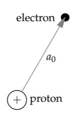
In the dimensional analysis of the size of hydrogen, the zeroth step is to give the size a name. The usual name and symbol for the radius of hydrogen is the Bohr radius a0.
The first step is to find the quantities that determine the size. That determination requires a physical model of hydrogen. A simple model is an electron orbiting a proton at a distance a0. Their electrostatic attraction provides the force F holding the electron in orbit:
\[F = \frac{e^{2}}{4 \pi \epsilon_{0}}\frac{1}{a^{2}_{0}},\]
where e is the electron charge. Our list of quantities should include the quantities in this equation; in that way, we teach dimensional analysis about what kind of force holds the atom together. Thus, we should somehow include e and \(\epsilon_{0}\). As when we estimated the power radiated by an accelerating charge (Section 5.4.3), we’ll include e and \(\epsilon_{0}\) as one quantity, \(e^{2}/4 \pi \epsilon_{0}\).
The force on the electron does not by itself determine the electron’s motion. Rather, the motion is determined by its acceleration. Computing the acceleration from the force requires the electron mass me, so our list should include me.
| \(a_{0}\) | L | size |
|---|---|---|
| \(e^{2}/4 \pi \epsilon_{0}\) | ML3T-2 | electrostatics |
| \(m_{e}\) | M | electron mass |
These three quantities made from three independent dimensions produce zero dimensionless groups (another application of the Buckingham Pi theorem introduced in Section 5.1.2). Without any dimensionless groups, we cannot say anything about the size of hydrogen. The lack of a dimensionless group tells us that our simple model of hydrogen is too simple.
There are two possible resolutions, each involving new physics that adds one new quantity to the list. The first possibility is to add special relativity by adding the speed of light c. That choice produces a dimensionless group and therefore a size. However, this size has nothing to do with hydrogen. Rather, it is the size of an electron, considering it as a cloud of charge (Problem 5.37).
The other problem with this approach is that electromagnetic radiation travels at the speed of light, so once the list includes the speed of light, the electron might radiate. As we found in Section 5.4.3, the power radiated by an accelerating charge is
\[P \sim \frac{q^{2}}{4 \pi \epsilon_{0}} \frac{a^{2}}{c^{3}}.\]
An orbiting electron is an accelerating electron (accelerating inward with the circular acceleration \(a = v^{2}/a_{0}\)), so the electron would radiate. Radiation would carry away energy from the electron, the electron would spiral into the proton, and hydrogen would not exist—nor would any other atom. So adding the speed of light only compounds our problem.
The second resolution is instead to add quantum mechanics. Its fundamental equation is the Schrödinger equation:
\[(-\frac{\hbar^{2}}{2m} \nabla^{2} + V) \psi = E \psi.\]
Most of the symbols in this partial-differential equation are not important for dimensional analysis—this disregard is how dimensional analysis simplifies problems. For dimensional analysis, the crucial point is that Schrödinger’s equation contains a new constant of nature: \(\hbar\), which is Planck’s constant h divided by \(2 \pi\). We can include quantum mechanics in our model of hydrogen simply by including \(\hbar\) on our list of relevant quantities. In that way, we teach dimensional analysis about quantum mechanics.
The new quantity \(\hbar\) is an angular momentum, which is a length (the lever arm) times linear momentum (mv). Therefore, its dimensions are
\[\underbrace{L}_{[r]} \times \underbrace{M}_{[m]} \times \underbrace{LT^{-1}}_{[v]} = ML^{2}T^{-1}.\]
The \(\hbar\) might save hydrogen. It contributes a fourth quantity without a fourth independent dimension. Therefore, it creates an independent dimensionless group.
| \(a_{0}\) | L | size |
|---|---|---|
| \(e^{2}/4\pi \epsilon_{0}\) | ML3T-2 | electrostatic mess |
| \(m_{e}\) | M | electron mass |
| \(\hbar\) | ML2T-1 | quantum |
To find it, look for a dimension appearing in only two quantities. Time appears in \(e^{2}/4 \pi \epsilon_{0}\) as \(T^{-2}\) and in \(\hbar\) as \(T^{-1}\). Therefore, the group contains the quotient \(\hbar^{2}/(e^{2}/4 \pi \epsilon_{0})\). Its dimensions are ML, which can be canceled by dividing by \(m_{e}a_{0}\). The resulting dimensionless group is
\[\frac{\hbar^{2}}{m_{e}a_{0}(e^{2}/4 \pi \epsilon_{0})}.\]
As the only independent dimensionless group, it must be a dimensionless constant. Therefore, the size (as the radius) of hydrogen is given by
\[a_{0} \sim \frac{\hbar^{2}}{m_{e}(e^{2}/4 \pi \epsilon_{0})}.\]
Now let’s plug in the constants. We could just look up each constant, but that approach gives exponent whiplash; the powers of ten swing up and down and end on a seemingly random value. To gain insight, we’ll instead use the numbers for the backs of envelopes (p. xvii). That table deliberately has no entry for \(\hbar\) by itself, nor for the electron mass me. Both omissions can be resolved with a symmetry operation (Problem 5.35).
Problem 5.35 Shortcuts for atomic calculations
Many atomic problems, such as the size or binding energy of hydrogen, end up in expressions with \(\hbar\), the electron mass me, and \(e^{2}/4 \pi \epsilon_{0}\). You can avoid remembering those constants by instead remembering the following values:
\[\hbar c \approx 200 eV nm = 2000 eV \mathring{A} \]
\[m_{e}c^{2} \sim 0.5 \times 10^{6} eV \: \textrm{(the electron rest energy)}\]
\[\frac{e^{2}/4 \pi \epsilon_{0}}{\hbar c} \equiv \alpha \approx 1/137 \: \textrm{(the fine-structure constant)}.\]
Use these values and dimensional analysis to find the energy of a photon of green light (which has a wavelength of approximately 0.5 micrometers), expressing your answer in electron volts.
In our expression for the Bohr radius, \(\hbar^{2}/m_{e}(e^{2}/4 \pi \epsilon_{0})\), we can replace \(\hbar\) with \(\hbar c\) and me with \(m_{e}c^{2}\) simultaneously: Multiply by 1 in the form \(c^{2}/c^{2}\); it is a convenient symmetry operation.
\[a_{0} \sim \frac{\hbar^{2}}{m_{e}(e^{2}/4 \pi \epsilon_{0})} \times \frac{c^{2}}{c^{2}} = \frac{(\hbar c)^{2}}{m_{e}c^{2}(e^{2}/4 \pi \epsilon_{0})}.\]
Now the table provides the needed values: for \(\hbar c\), \(m_{e}c^{2}\), and \(e^{2}/4 \pi \epsilon_{0}\). However, we can make one more simplification because the electrostatic mess \(e^{2}/4 \pi \epsilon_{0}\) is related to a dimensionless constant. To see the relation, multiply and divide by \(\hbar c\):
\[\frac{e^{2}}{4 \pi \epsilon_{0}} = \underbrace{(\frac{e^{2}/4\pi \epsilon_{0}}{\hbar c})}_{\alpha} \hbar c.\]
The factor in parentheses is known as the fine-structure constant \(\alpha\); it is a dimensionless measure of the strength of electrostatics, and its numerical value is close to 1/137 or roughly 0.7 ×10⁻². Then
\[\frac{e^{2}}{4 \pi \epsilon_{0}} = \alpha \hbar c.\]
This substitution further simplifies the size of hydrogen:
\[a_{0} \sim \frac{(\hbar c)^{2}}{m_{e}c^{2} \times e^{2}/4 \pi \epsilon_{0}} = \frac{(\hbar c)^{2}}{m_{e}c^{2} \times \alpha \hbar c} = \frac{\hbar c}{\alpha \times m_{e}c^{2}}.\]
Only now, having simplified the calculation down to abstractions worth remembering (\(\alpha\), \(m_{e}c^{2}\), and \(\hbar c\)), do we plug in the entries from the table.
\[a_{0} \sim \frac{\overbrace{200 eV nm}^{\hbar c}}{\underbrace{0.7 \times 10^{-2}}_{\alpha} \times \underbrace{5 \times 10^{5} eV}_{m_{e}c^{2}}}.\]
This calculation we can do mentally. The units of electron volts cancel, leaving only nanometers (nm). The two powers of ten upstairs (in the numerator) and the three powers of ten downstairs (in the denominator) result in 10−1 nanometers or 1 ångström (10−10 meters). The remaining factors result in a factor of 1/2: 2/(0.7 × 5) ≈ 1/2.
Therefore, the size of hydrogen—the Bohr radius—is about 0.5 ångströms:
\[a_{0} \sim 0.5 \times 10^{-10} m = 0.5 \mathring{A}.\]
Amazingly, the missing dimensionless prefactor is 1. Thus, atoms are ångström-sized. Indeed, hydrogen is 1 ångström in diameter. All other atoms, which have more electrons and therefore more electron shells, are larger. A useful rule of thumb is that a typical atomic diameter is 3 ångströms.
What binding energy does this size produce?
The binding energy is the energy required to disassemble the atom by removing the electron and dragging it to infinity. This energy, denoted E0, should be roughly the electrostatic energy of a proton and electron separated by the Bohr radius a0:
\[E_{0} \sim \frac{e^{2}}{4 \pi \epsilon_{0}} \frac{1}{a_{0}}.\]
With our result for a0, the binding energy becomes
\[E_{0} \sim m_{e} (\frac{e^{2}}{4 \pi \epsilon_{0}})^{2} \frac{1}{\hbar^{2}}.\]
The missing dimensionless prefactor is just 1/2:
\[E_{0} = \frac{1}{2} m_{e} (\frac{e^{2}}{4 \pi \epsilon_{0}})^{2} \frac{1}{\hbar^{2}}.\]
Problem 5.36 Shortcut to calculate the binding energy of hydrogen
Use the shortcuts in Problem 5.35 to show that the binding energy of hydrogen is roughly 14 electron volts. From your symbolic expression for the energy, which is also the kinetic energy of the electron, estimate its speed as a fraction of c.
In Problem 5.36, you showed, using the values of \(\hbar c\), \(m_{e}c^{2}\), and \(\alpha\), that this energy is roughly 14 electron volts. For the sake of a round number, let’s call the binding energy roughly 10 electron volts.
This energy sets the scale for chemical bonds. In Section 3.2.1, we calculated, by unit conversion, that 1 electron volt per molecule corresponded to roughly 100 kilojoules per mole. Therefore, breaking a chemical bond requires roughly 1 megajoule per mole (of bonds). As a rough estimate, it is not far off. For example, if the molecule consists of a few life-related atoms (carbon, oxygen, and hydrogen), then the molar mass is roughly 50 grams—a small jelly donut. Therefore, burning a jelly donut, as our body does slowly when we eat the donut, should produce roughly 1 megajoule—a useful rule of thumb and way of imagining a megajoule.
Problem 5.37: Adding the speed of light
If we assume that a0 depends on \(e^{2}/4 \pi \epsilon_{0}\), me, and c, what size would dimensional analysis predict for hydrogen? This size is called the classical electron radius and denoted r0. How does it compare to the actual Bohr radius?
Problem 5.38: Thermal expansion
Estimate a typical thermal-expansion coefficient, also denoted \(\alpha\). It is defined as
\[\alpha \equiv \frac{\textrm{fractional change in a substance's length}}{\textrm{change in temperature}}.\]
The thermal-expansion coefficient depends on the binding energy E0. Assuming E0 ~ 10 eV, compare your estimate for \(\alpha\) with its value for everyday substances.
Provlem 5.39: Diffraction in the eye
Light passing through an opening, such as a telescope aperture or the pupil in the eye, diffracts (spreads out). By estimating the diffraction angle \(\theta\), we will be able to understand aspects of the design of the eye.
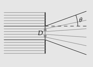
a. What are the valid dimensionless relations connecting the diffraction angle \(\theta\), the light wavelength \(\lambda\), and the pupil diameter D?
b. Diffraction is the result of the photons in the beam acquiring a vertical momentum \(\Delta p_{y}\). What is the scaling exponent \(\beta\) in \(\theta \: \alpha \: (\Delta p_{y})^{\beta}\)?
c. The Heisenberg uncertainty principle from quantum mechanics says that the uncertainty in the photon’s vertical momentum \(\Delta p_{y}\) is inversely proportional to the pupil diameter D. What is therefore the scaling exponent \(\gamma\) in \(\theta \: \alpha \: D^{\gamma}\)?
d. Therefore find \(\theta\) as a function of \(\lambda\) and D.
e. Estimate a pupil diameter and the resulting diffraction angle. The light-sensitive cells in the retina that we use in bright light are the cones. They are most dense in the fovea—the central region of the retina that we use for reading and any other task requiring sharp vision. At that location, their density is roughly 0.5×10⁷ per square centimeter. Is that what you would predict?
Problem 5.40: Kepler's third law for non-inverse-square force laws
With an inverse-square force, Kepler’s third law—the relation between orbit radius and period—is \(T \: \propto \: r^{3/2}\) (Section 4.2.2). Now generalize the law to forces of the form \(F \: \propto \: r^{n}\), using dimensional analysis to find the scaling exponent \(\beta\) in the orbital period \(T \: \propto \: r^{\beta}\) as a function of the scaling exponent n in the force law.
Problem 5.41: Ground state energy for general potentials
Just as we can apply dimensional analysis to classical orbits (Problem 5.40), we can apply it to quantum orbits. When the force law is \(F \: \propto \: r^{-2}\) (electrostatics), or the potential is \(V \: \propto \: r^{-1}\), we have hydrogen, for which we estimated the binding or ground-state energy. Now generalize to potentials where \(V = Cr^{\beta}\).
The relevant quantities are the ground-state energy E0, the proportionality constant C in the potential, the quantum constant \(\hbar\), and the particle’s mass m. These four quantities, built from three dimensions, form one independent dimensionless group. But it is not easy to find. Therefore, use linear algebra to find the exponents \(\gamma\), \(\delta\), and \(\epsilon\) that make \(E_{0}C^{\gamma}\hbar^{\delta}m^{\epsilon}\) dimensionless. In the case \(\beta = -1\) (electrostatics), check that your result matches our result for hydrogen.
5.5.2 Blackbody radiation
With quantum mechanics and its new constant \(\hbar\), we can explain the surface temperatures of planets or even stars. The basis is blackbody radiation: A hot object—a so-called blackbody—radiates energy. (Here, “hot” means warmer than absolute zero, so every object is hot.) Hotter objects radiate more, so the radiated energy flux F depends on the object’s temperature T.
How are the energy flux \(F\) and the surface temperature \(T\) connected?
I stated the connection in Section 4.2, but now we know enough dimensional analysis to derive almost the entire result without a detailed study of the quantum theory of radiation. Thus, let’s follow the steps of dimensional analysis to find F, and start by listing the relevant quantities.
The list begins with the goal, the energy flux F. Blackbody radiation can be understood properly through the quantum theory of radiation, which is the marriage of quantum mechanics to classical electrodynamics. (A diagram of the connection, which requires the subsequent tool of easy cases, is in Section 8.4.2.) For the purposes of dimensional analysis, this theory supplies two constants of nature: \(\hbar\) from quantum mechanics and the speed of light c from classical electrodynamics. The list also includes the object’s temperature T, so that dimensional analysis knows how hot the object is; but we’ll include it as the thermal energy \(k_{B}T\).
The four quantities built from three independent dimensions produce one independent dimensionless group. Our usual route to finding this group, by looking for dimensions that appear in only one or two variables, fails because mass, like length, appears in three quantities, and time appears in all four. An alternative is to apply linear algebra, as you practiced in Problem 5.41. But it is messy.
A less brute-force and more physically meaningful alternative is to choose a system of units where \(c \equiv 1\) and \(\hbar \equiv 1\). Each of these two choices has a physical meaning. Before using the choices, it is worth understanding these meanings. Otherwise we are back to pushing symbols around.
The first choice, \(c \equiv 1\), expresses the unity of space and time embedded and embodied in Einstein’s theory of special relativity. With \(c \equiv 1\), length and time have the same dimensions and are measured in the same units. We can then say that the Sun is 8.3 minutes away from the Earth. That time is equivalent to the distance of 8.3 light minutes (the distance that light travels in 8.3 minutes).
The choice \(c \equiv 1\) also expresses the equivalence between mass and energy. We use this choice implicitly when we say that the mass of an electron is 5 × 10⁵ electron volts—which is an energy. The complete statement is that, in the usual units, the electron’s rest energy \(m_{e}c^{2}\) is 5 × 10⁵ electron volts. But when we choose \(c \equiv 1\), then 5×10⁵ electron volts is also the mass me.
The second choice, \(\hbar \equiv 1\), expresses the fundamental insight of quantum mechanics, that energy is (angular) frequency. The complete connection between energy and frequency is
\[E = \hbar \omega\]
When \(\hbar \equiv 1 \), then E is \(\omega\).
These two unit choices implicitly incorporate their physical meanings into our analysis. Furthermore, the choices so simplify our table of dimensions that we can find the proportionality between flux and temperature without any linear algebra.
First, choosing \(c \equiv 1\) makes the dimensions of length and time equivalent:
\[c \equiv 1 \: \textrm{implies} \: L \equiv T.\]
Thus, in the table we can replace T with L.
Then adding the choice \(\hbar \equiv 1\) contributes the dimensional equation
\[\underbrace{ML^{2}T^{-2}}_{[E]} \equiv \underbrace{T^{-1}}_{[\omega]}\]
It looks like a useless mess; however, replacing T with L (from \(c \equiv 1\)) simplifies it:
\[M \equiv L^{-1}.\]
In summary, setting \(c \equiv 1\) and \(\hbar \equiv 1\) makes length and time equivalent dimensions and makes mass and inverse length equivalent dimensions.
With these equivalences, let’s rewrite the table of dimensions, one quantity at a time.
1. Flux F. Its dimensions, in the usual system, were MT−3. In the new system, T−3 is equivalent to M3, so the dimensions of flux become M4.
2. Thermal energy \(k_{B}T\). Its dimensions were ML2T−2. In the new system, T−2 is equivalent to L−2, so the dimensions of thermal energy become M. And they should: Choosing \(c \equiv 1\) makes energy equivalent to mass.
3. Quantum constant \(\hbar\). By fiat (when we chose \(\hbar \equiv 1\)), it is now dimensionless and just 1, so we do not list it.
4. Speed of light c. Also by fiat, c is just 1, so we do not list it either
Our list has become shorter and the dimensions in it simpler. In the usual system, the list had four quantities (F, \(k_{B}T\), \(\hbar\), and c) and three independent dimensions (M, L, and T). Now the list has only two quantities (F and kBT) and only one independent dimension (M). In both systems, there is only one dimensionless group.
| F | M4 | energy flux |
| kBT | M | thermal energy |
In the usual system, the Buckingham Pi calculation is as follows:
4 quantities
- 3 independent dimensions
___________________________
1 independent dimensionless group
In the new system, the calculation is
2 quantities
- 1 independent dimension
_____________________________
1 independent dimensionless group
(If the number of independent dimensionless groups had not been the same, we would know that we had made a mistake in converting to the new system.) In the simpler system, the independent dimensionless group proportional to F is now almost obvious. Because F contains M4 and kBT contains M1, the group is just \(F/(k_{B}T)^{4}\).
Alas, no lunch is free and no good deed goes unpunished. Now we pay the price for the simplicity: We have to restore c and \(\hbar\) in order to find the equivalent group in the usual system of units. Fortunately, the restoration doesn’t require any linear algebra.
The first step is to compute the usual dimensions of \(F/(k_{B}T)^{4}\):
\[[\frac{F}{(k_{B}T)^{4}}] = \frac{MT^{-3}}{(ML^{2}T^{-2})^{4}} = M^{-3}L^{-8}T^{-5}.\]
The rest of the analysis for making this quotient dimensionless just rolls downhill without our needing to make any choices. The only way to get rid of M−3 is to multiply by \(\hbar^{3}\): Only \(\hbar\) contains a dimension of mass.
The result has dimensions L−2T2:
\[[\frac{F}{(k_{B}T)^{4}}\hbar^{3}] = \underbrace{M^{-3}L^{-8}T^{-5}}_{[F/(k_{B}T)^{4}]} \times \underbrace{(ML^{2}T^{-1})^{3}}_{[\hbar]} = L^{-2}T^{2}.\]
To clear these dimensions, multiply by c2. The independent dimensionless group proportional to F is therefore
\[\frac{F \hbar^{3}c^{2}}{(k_{B}T)^{4}}.\]
As the only independent dimensionless group, it is a constant, so
\[F \sim \frac{(k_{B}T)^{4}}{\hbar^{3}c^{2}}.\]
Including the dimensionless prefactor hidden in the twiddle (~),
\[F = \underbrace{\frac{\pi^{2}}{60} \frac{k_{B}^{4}}{\hbar^{3}c^{2}}}_{\sigma} T^{4}.\]
This result is the Stefan–Boltzmann law, and all the constants are lumped into \(\sigma\), the Stefan–Boltzmann constant:
\[\sigma \equiv \frac{\pi^{2}}{60} \frac{k_{B}^{4}}{\hbar^{3}c^{2}}.\]
In Section 4.2.1, we used the scaling exponent in the Stefan–Boltzmann law to estimate the surface temperature of Pluto: We started from the surface temperature of the Earth and used proportional reasoning. Now that we know the full Stefan–Boltzmann law, we can directly calculate a surface temperature. In Problem 5.43, you will estimate the surface temperature of the Earth (and you then try to explain the life-saving discrepancy between prediction and reality). Here, we’ll estimate the surface temperature of the Sun using the Stefan–Boltzmann law, the solar flux at the top of the Earth’s atmosphere, and proportional reasoning.
Let’s work backward from our goal toward what we know. We would like to find the Sun’s surface temperature TSun. If we knew the energy flux FSun at the Sun’s surface, then the Stefan–Boltzmann law would give us the temperature:
\[T_{Sun} = (\frac{F_{Sun}}{\sigma})^{1/4}.\]
We can find FSun from the solar flux F at the Earth’s orbit by using proportional reasoning. Flux, as we argued in Section 4.2.1, is inversely proportional to distance squared, because the same energy flow (a power) gets smeared over a surface area proportional to the square of the distance from the source. Therefore,
\[\frac{F_{\textrm{Sun's surface}}}{F} = (\frac{r_{\textrm{Earth's orbit}}}{R_{\textrm{Sun}}})^{2},\]
where RSun is the radius of the Sun. A related distance ratio is
\[\frac{D_{Sun}}{r_{\textrm{Earth's orbit}}} = \frac{2R_{Sun}}{r_{\textrm{Earth's orbit}}},\]
where DSun is the diameter of the Sun. This ratio is the angular diameter of the Sun, denoted \(\theta_{Sun}\). Therefore,
\[\frac{r_{\textrm{Earth's orbit}}}{R_{Sun}} = \frac{2}{\theta_{Sun}}.\]
From a home experiment measuring the angular diameter of the Moon, which has the same angular diameter as the Sun, or from the table of constants, the angular diameter \(\theta_{Sun}\) is approximately 10−2. Therefore, the distance ratio is approximately 200, and the flux ratio is approximately 2002 or 4×10⁴.
Continuing to unwind the reasoning chain, we get the flux at the Sun’s surface:
\[F_{\textrm{Sun's surface}} \approx 4 \times 10^{4} \times \underbrace{1300 W m^{-2}}{F} \approx 5 \times 10^{7} W m^{-2}.\]
This flux, from the Stefan–Boltzmann law, corresponds to a surface temperature of roughly 5400 K
\[T_{Sun} \approx (\frac{5 \times 10^{7}Wm^{-2}}{6 \times 10^{-8}Wm^{-2}K^{-4}})^{1/4} \approx 5400K.\]
This prediction is quite close to the measured temperature of 5800 K.
Problem 5.42: Redo the blackbody-radiation analysis using linear algebra
Use linear algebra to find the exponents y, z, and w that make the combination \(F \times (k_{B}T)^{y}\hbar^{z}c^{w}\) dimensionless.
Problem 5.43: Blackbody temperature of the Earth
Use the Stefan–Boltzmann law \(F = \sigma T^{4}\) to predict the surface temperature of the Earth. Your prediction should be somewhat colder than reality. How do you explain the (life-saving) difference between prediction and reality?
Problem 5.44: Lengths related by the fine-structure constant
Arrange these important atomic-physics lengths in order of increasing size:
a. the classical electron radius (Problem 5.37) \(r_{0} \equiv (e^{2}/4 \pi \epsilon_{0})/m_{e}c^{2}\) (roughly the radius of an electron if its rest energy were entirely electrostatic energy).
b. the Bohr radius a0 from Section 5.5.1.
c. the reduced wavelength \(\lambda\) of a photon with energy 2E0, where \(\cancel{\lambda} \equiv \lambda/2\pi\) (analogously to how \(\hbar \equiv h/2 \pi\) or \(f = \omega/2\pi\)) and E0 is the binding energy of hydrogen. (The energy 2E0, also the absolute value of the potential energy in hydrogen, is called the Rydberg).
d. the reduced Compton wavelength of the electron, defined as \(\hbar/m_{e}c\).
Place the lengths on a logarithmic scale, and label the gaps (the ratios of successive lengths) in terms of the fine-structure constant \(\alpha\).
5.5.3 Molecular binding energies
We studied hydrogen, which as an element scarcely exists on Earth, mainly to understand chemical bonds. Chemical bonds are formed by attractions between electrons and protons, so the hydrogen atom is the simplest chemical bond. The main defect of this model is that the electron–proton bond in a hydrogen atom is much shorter than in most bonds. A typical chemical bond is roughly 1.5 ångströms, three times larger than the Bohr radius. Because electrostatic energy scales as \(E \: \alpha \: 1/r\), a typical bond energy should be smaller than hydrogen’s binding energy by a factor of 3. Hydrogen’s binding energy is roughly 14 electron volts, so Ebond is roughly 4 electron volts—in agreement with the bond-energy values tabulated in Section 2.1.
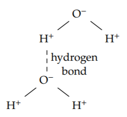
Another important bond is the hydrogen bond. These intermolecular bonds, which hold water molecules together, are weaker than the intramolecular hydrogen–oxygen bonds within a water molecule. But hydrogen bonds determine important properties of the most important liquid on our planet. For example, the hydrogen-bond energy determines water’s heat of vaporization—which determines much of our weather, including the average rainfall on the Earth (as we found in Section 3.4.3).
To estimate the strength of hydrogen bonds, use the proportionality
\[E_{electrostatic} \alpha \frac{q_{1}q_{2}}{r}.\]
A hydrogen bond is slightly longer than a typical bond. Instead of the typical 1.5 ångströms, it is roughly 2 ångströms. The bond length is in the denominator, so the greater length reduces the bond energy by a factor of 4/3.
Furthermore, the charges involved, q1 and q2, are smaller than the charges in a regular, intramolecular bond. A regular bond is between a full proton and a full electron of charge. A hydrogen bond, however, is between the excess charge on oxygen and the corresponding charge deficit on hydrogen. The excess and deficit are significantly smaller than a full charge. On oxygen the excess may be 0.5e (where e is the electron charge). On each hydrogen, because of conservation, it would then be 0.25e. These reductions in charge contribute factors of 1/2 and 1/4 to the hydrogen-bond energy. The resulting energy is roughly 0.4 electron volts:
\[4eV \times \frac{3}{4} \times \frac{1}{2} \times \frac{1}{4} \approx 0.4 eV.\]
This estimate is not bad considering the rough numbers that it used. Empirically, a typical hydrogen bond is 23 kilojoules per mole or about 0.25 electron volts. Each water molecule forms close to four hydrogen bonds (two from the oxygen to foreign hydrogens, and one from each hydrogen to a foreign oxygen). Thus, each molecule gets credit for almost two hydrogen bonds—one-half of the per-molecule total in order to avoid counting each bond twice. Per water molecule, the result is 0.4 electron volts
Because vaporizing water breaks the hydrogen bonds, but not the intramolecular bonds, the heat of vaporization of water should be approximately 0.4 electron volts per molecule. In macroscopic units, it would be roughly 40 kilojoules per mole—using the conversion factor from Section 3.2.1, that 1 electron volt per molecule is roughly 100 kilojoules per mole.
Because the molar mass of water is 1.8×10⁻² kilograms, the heat of vaporization is also 2.2 megajoules per kilogram:
\[\frac{40kJ}{mol} \times \frac{1mol}{1.8 \times 10^{-2} kg} \approx \frac{2.2 \times 10^{6} J}{kg}.\]
And it is (p. xvii). We used this value in Section 3.4.3 to estimate the average worldwide rainfall. The amount of rain, and so the rate at which many plants grow, is determined by the strength of hydrogen bonds.
Problem 5.45: Rotational energies
The quantum constant \(\hbar\) is also the smallest possible angular momentum of a rotating system. Use that information to estimate the rotational energy of a small molecule such as water (in electron volts). To what electromagnetic wavelength does this energy correspond, and where in the electromagnetic spectrum does it lie (for example, radio waves, ultraviolet, gamma rays)?
5.5.4 Stiffness and sound speeds
An important macroscopic consequence of the per-atom and per-molecule energies is the existence of solid matter: substances that resist bending, twisting, squeezing, and stretching. These resistance properties are analogous to spring constants.
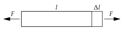
However, a spring constant is not the quantity to estimate first, because it is not invariant under simple changes. For example, a thick bar resists stretching more than a thin bar does. Similarly, a shorter bar resists stretching more than a longer bar does. The property independent of the shape or amount of substance—invariant to these changes—is the stiffness or elastic modulus. There are several elastic moduli, of which the Young’s modulus is the most broadly useful. It is defined by
\[Y = \frac{\textrm{stress } \sigma \textrm{ applied to the substance}}{\textrm{fractional change in its length } [(\Delta l)(l)]}.\]
The ratio in the denominator occurs so often that it has its own name and symbol: the strain \(\epsilon\).
Stress, like the closely related quantity pressure, is force per area: It is the applied force F divided by the cross-sectional area. The denominator, the fractional change in length, is the dimensionless ratio \((\Delta l)/l\). Thus, the dimensions of stiffness are the dimensions of pressure—which are also the dimensions of energy density. To see the connection between pressure and energy density, multiply the definition of pressure (force per area) by length over length:
\[\textrm{pressure} = \frac{\textrm{force}}{\textrm{area}} \times \frac{\textrm{length}}{\textrm{length}} = \frac{\textrm{energy}}{\textrm{volume}}.\]
As energy per volume, we can estimate a typical elastic modulus Y. For the numerator, a suitable energy is the typical binding energy per atom—the energy Ebinding required to remove the atom from the substance by breaking its bonds to surrounding atoms. For the denominator, a suitable volume is a typical atomic volume a3, where a is a typical interatomic spacing (3 ångströms). The result is
\[Y \sim \frac{E_{binding}}{a^{3}}.\]
This derivation is slightly incomplete: In multiplying the definition of pressure by length over length, we knew only that the two lengths have the same dimensions, but not whether they have comparable values. If they do not, then the estimate for Y needs a dimensionless prefactor, which might be far from 1. Therefore, before we estimate Y, let’s confirm the estimate by using a second method, an analogy—a form of abstraction that we learned in Section 2.4.
The analogy, with which we also began this discussion of stiffness, is between a spring constant (k) and a Young’s modulus (Y). There are three physical quantities in the analogy.
1. Stiffness. For a single spring, we measure stiffness using k. For a material, we use the Young’s modulus Y. Therefore, k and Y are analogous.
2. Extension. For a single spring, we measure extension using the absolute length change \(\Delta x\). For a material, we use the fractional length change \((\Delta l)/l\) (the strain \(\epsilon\)). Therefore, \(\Delta x\) and \((\Delta l)/l\) are analogous.
3. Energy. For a single spring, we measure energy using the energy E directly. For a material, we use an intensive quantity, the energy density \(\varepsilon \equiv \frac{E}{V}\). Therefore, E and \(\varepsilon\) are analogous.
Because the energy in a spring is
\[E \sim k (\Delta x)^{2},\]
by analogy the energy density in a material will be
\[\epsilon \sim Y(\frac{\Delta{l}}{l})^{2}.\]
Let’s estimate Y by setting \(\Delta l \sim l\). Physically, this choice means stretching or compressing each bond by its own length. This harsh treatment is, as a reasonable assumption, sufficient to break the bond and release the binding energy. Then the right side becomes simply the Young’s modulus Y.
The left side, the energy density, becomes simply the bond energy per volume. For the volume, if we use the volume of one atom, roughly a3, then the bond energy contained in this volume is the binding energy of one atom. Then the Young’s modulus becomes
\[Y \sim \frac{E_{binding}}{a^{3}}.\]
This result is what we predicted based on the dimensions of pressure. However, we now have a physical model of the Young’s modulus, based on an analogy between it and spring constant.
Having arrived at this conclusion from dimensions and from an analogy, let’s apply it to estimate a typical Young’s modulus. To estimate the numerator, the binding energy, start with the typical bond energy of 4 electron volts per bond. With each atom is connected to, say, five or six other atoms, the total energy is roughly 20 electron volts. Because bonds are connections between pairs of atoms, this 20 electron volts counts each bond twice. Therefore, a typical binding energy is 10 electron volts per atom.
Using a ~ 3 ångströms, a typical stiffness or Young’s modulus is
\[Y \sim \frac{E_{binding}}{a^{3}} \sim \frac{10eV}{(3 \times 10^{-10} m)^{3}} \times \frac{1.6 \times 10^{-19}J}{eV} \sim \frac{1}{2} \times 10^{11} J m^{-3}.\]
For very rough estimates, a convenient value to remember is 1011 joules per cubic meter. Because energy density and pressure have the same dimensions, this energy density is also 1011 pascals or 106 atmospheres. (Because atmospheric pressure is only 1 atmosphere, a factor of 1 million smaller, it has little effect on solids.)
| Y (1011 Pa) | |
| diamond | 12 |
| steel | 2 |
| Cu | 1.2 |
| Al | 0.7 |
| glass | 0.6 |
| granite | 0.3 |
| Pb | 0.18 |
| concrete | 0.17 |
| oak | 0.1 |
| ice | 0.1 |
Using a typical stiffness, we can estimate sound speeds in solids. The speed depends not only on the stiffness, but also on the density: denser materials respond more slowly to the forces due to the stiffness, so sound travels more slowly in denser substances. From stiffness \(Y\) and density \(\rho\), the only dimensionally correct way to make a speed is \(\sqrt{Y/\rho}\). If this speed is the speed of sound, then
\[c_{s} \sim \sqrt{\frac{Y}{\rho}}.\]
Based on a typical Young’s modulus of 0.5×10¹¹ pascals and a typical density of 2.5 × 10³ kilograms per cubic meter (for example, rock), a typical speed of sound is 5 kilometers per second:
\[c_{s} \sim \sqrt{\frac{0.5 \times 10^{11} Pa}{2.5 \times 10^{3} kg m^{-3}}} \approx 5 km s^{-1}.\]
This prediction is reasonable for most solids and is exactly correct for steel! With this estimate, we end our dimensional-analysis tour of the properties of materials. Look what dimensional analysis, combined with analogy and proportional reasoning, has given us: the size of atoms, the energies of chemical bonds, the stiffness of materials, and the speed of sound.