8.2: Linear Optimization

Linear optimization is a method applicable for the solution of problems in which the objective function and the constraints appear as linear functions of the decision variables. The constraint equations may be in the form of equalities or inequalities[1]. In other words, linear optimization determines the way to achieve the best outcome (for example, to maximize profit or to minimize cost) in a given mathematical model and given some lists of requirements represented as linear equations [2].

Applications

Linear optimization can be applied to numerous fields, in business or economics situations, and also in solving engineering problems. It is useful in modeling diverse types of problems in planning, routing, scheduling, assignment and design [2].

Some examples of applications in different industries

Petroleum refineries

One of the early industrial applications of linear optimization has been made in the petroleum refineries. An oil refinery has a choice of buying crude oil from different sources with different compositions at different prices. It can manufacture different products, such as diesel fuel, gasoline and aviation fuel, in varying quantities. A mix of the purchased crude oil and the manufactured products is sought that gives the maximum profit.

Manufacturing firms

The sales of a firm often fluctuate, therefore a company has various options. It can either build up an inventory of the manufactured products to carry it through the period of peak sales, or to pay overtime rates to achieve higher production during periods of high demand. Linear optimization takes into account the various cost and loss factors and arrive at the most profitable production plan.

Food-processing industry

Linear optimization has been used to determine the optimal shipping plan for the distribution of a particular product from different manufacturing plants to various warehouses.

Telecommunications

The optimal routing of messages in a communication network and the routing of aircraft and ships can also be determined by linear optimization method.

Characteristics of Linear Optimization

The characteristics of a linear optimization problem are:

1. The objective function is of the minimization type
2. All the constraints are of the equality type
3. All the decision variables are non-negative

Any linear optimization problem can be expressed in the standard form by using the following transformation:

1) The maximization of a function \(f\left(x_{1}, x_{2}, \ldots, x_{n}\right)\) is equivalent to the minimization of the negative of the same function.

For example:

Minimize

\[f=c_{1} x_{1}+c_{2} x_{2}+\ldots+c_{n} x_{n}\nonumber \]

is equivalent to

Maximize

\[f^{\prime}=-f=-c_{1} x_{1}-c_{2} x_{2}-\ldots-c_{n} x_{n}\nonumber \]

Consequently, the objective function can be stated in the minimization form in any linear optimization problem.

2) If a constraint appears in the form of a "less than or equal to" type of inequality as

\[a_{k 1} x_{1}+a_{k 2} x_{2}+\ldots+a_{k n} x_{n} \leq b_{k}\nonumber \]

it can be converted into the equality form by adding a non-negative slack variable as follows:

\[a_{k 1} x_{1}+a_{k 2} x_{2}+\ldots+a_{k n} x_{n}+x_{n+1}=b_{k}\nonumber \]

Similarly, if the constraint is in the form of a "greater than or equal to" type of inequality, it can be converted into the equality form by subtracting the surplus variable .

3) In most engineering optimization problems, the decision variables represent some physical dimensions, hence the variables will be non-negative.

However, a variable may be unrestricted in sign in some problems. In such cases, an unrestricted variable (which can take a positive, negative or zero value) can be written as the difference of two non-negative variables.

Thus, if is unrestricted in sign, it can be written as \(x_{j}=x_{j}^{\prime}-x_{j}^{\prime \prime}\), where

\(0 \leq x_{j}^{\prime}\) and \(0 \leq x_{j}^{\prime \prime}\)

It can be seen that will be negative, zero or positive, depending on whether is greater than, equal to, or less than

Example \(\PageIndex{1}\)

This example comes from Seborg, Edgar, and Mellinchamp (with some corrections). A chemical company is mixing chemical component, \(A\) and \(B\) to produce product, \(E\) and \(F\). The chemical reaction is listed below:

\[A+B=E\nonumber \]

\[A+2 B=F\nonumber \]

The conditions of this production is listed as below:

	Cost of Materials	Maximum Available per day	Fixed Cost
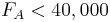
A	$0.15/lbs	40,000lbs	350
B	$0.20/lbs	30,000lbs	200
	Value of Products	Maximum Production Rate
E	$0.40/lbs	30,000lbs
F	$0.33/lbs	30,000lbs

The profit of this production can be simply described as the function below:

Profit

=	∑	FsVs −	∑	FrVr − C.P. − F.C.
	s		r

• Flow Rates of Products
• Flow Rates of Raw Materials
• Values of Products
• Values of Raw Materials
• Cost of Production
• Fixed Cost

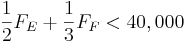
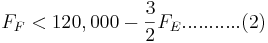
Constraints

• :
• :
• :
• :
• : ≥

Solution

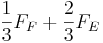
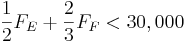
\[F_{A}=\frac{1}{2} F_{E}+\frac{1}{3} F_{F} \nonumber \]

\[F_{B}=\frac{1}{2} F_{E}+\frac{2}{3} F_{F} \nonumber \]

\[\text { Profit }=\sum_{s} F_{s} V_{s}-\sum_{r} F_{r} V_{r}-C . P .-F . C . \nonumber \]

\[=\left(0.4 \psi_{F_{j}}+0.33 F_{F^{-}}\right)-\left(0.15 F_{A}^{\prime}-0.2 F_{H}^{\prime}\right)-\left(0.15 F_{F_{i}}+0.05 F_{F}^{\prime}\right)-(350+200 i \nonumber \]

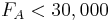
0 " src="/@api/deki/files/18014/image-717.png">

0 " src="/@api/deki/files/18016/image-718.png">

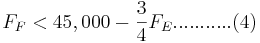
-\frac{3}{2} F_E ...........(1) " src="/@api/deki/files/18018/image-719.png">

0 " src="/@api/deki/files/18025/image-723.png">

0 " src="/@api/deki/files/18027/image-724.png">

-\frac{3}{4} F_E ...........(3) " src="/@api/deki/files/18029/image-725.png">

Solution using Mathematica

INPUT:

profit = 0.25 FE + 0.28 FF - 0.15 FA - 0.2 FB - 350 - 200

sol = Maximize[ profit, {FA > 0, FB > 0, FA < 40000, FB < 30000, FE > 0, FE < 30000, FF > 0, FF < 30000, FA == (1/2) FE + (1/3) FF, FB == (1/2) FE + (2/3) FF}, {FE, FF}]

OUTPUT: {3875., {FE -> 30000., FF -> 22500.}}

Solution using "Solver" in Excel.

Result is FE = 30,000, FF = 22500.

If only process ! or process 2 were running a full capacity, the profit would be less.

Linear Optimization

The above is an example of linear optimization. It is often used in oil refinery to figure out maximal profit in response to market competition.

2.4.4 Graph

Example 2

Example of Linear Optimization Problem in Excel

Written by: Jennifer Campbell, Katherine Koterba, MaryAnn Winsemius

Part 1: Organize Given Information

As stated in the Linear Optimization section example above, there are three categories of information needed for solving an optimization problem in Excel: an objective function, constraints, and decision variables.

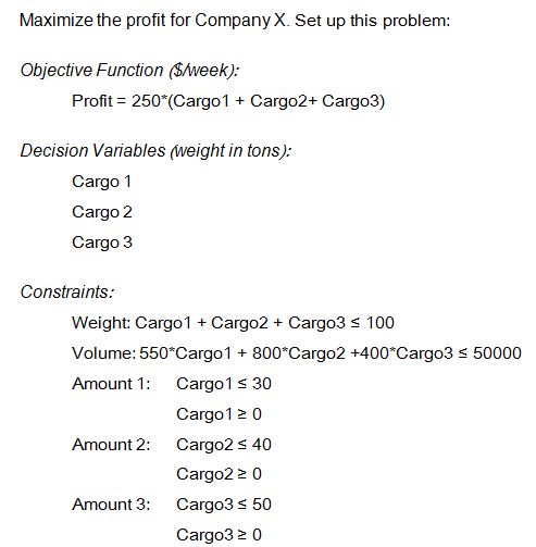
We will use the following example to demonstrate another application of linear optimization. We will be optimizing the profit for Company X’s trucking business.

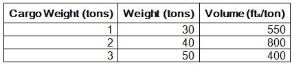
To reach capacity, Company X must move 100 tons of cargo per day by truck. Company X’s trucking fee is $250/ton. Besides the weight constraint, the company can only move 50,000 ft^3 of cargo per day due to limited volume trucking capacity. The following amounts of cargo are available for shipping each day:

Part 2: Set Up the Problem Using Excel

Solver is an Add-in for Microsoft Excel. It will be used to optimize Company X’s profit. If ‘Solver’ is not on the ‘Tools’ menu in Excel, then use the following steps to enable it:

For Windows 2007:

• Click on the Office button at the top left corner of the screen. Click on the “Excel Options” button on the bottom right of the menu.
• Select “Add-ins.” Make sure that “Excel Add-ins” is selected in the “Manage” drop down list. Click “Go.”
• A new window will appear entitled “Add-ins.” Select “Solver Add-in” by checking the box. Click “Go.”
• A Configuration window will appear. Allow Office to install the Add-in.
• The solver has been successfully installed. (See Windows Help for more instruction.)

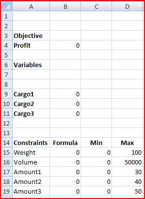
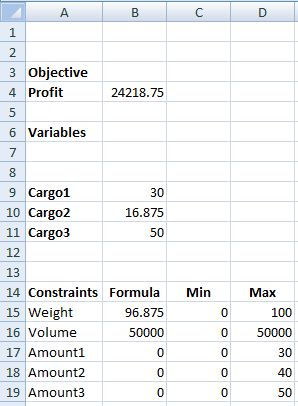
Use the figure below to set up your Excel worksheet.

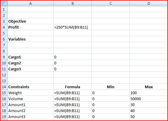
Enter in the following formulas to the cells as shown below:

Part 3: Running Solver

• Click on the “Data” tab and select “Solver”. A dialog box will appear.
• Enter the parameters as shown in the figure below.

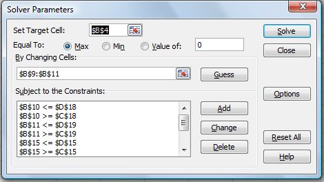
Detailed steps are as follows:

• In “Set Target Cell,” enter the cell corresponding to the company’s profit (B4).
• Select “Max” under “Equal To.”
• Click on the “Options” tab and check the “Assume Linear Model” box.
• For “By Changing Cells:” select the cells in column B corresponding the cargo amounts (B9, B10, B11).

• To add constraints, select “Add” under “Subject to the Constraints” A dialog box will open.
• In the “Cell Reference:” field, enter the cell location of the decision value that is subject to constraint (i.e. B9).
• Use the pull-down menu in the middle to select the appropriate inequality relation (i.e. <=)
• In the “Constraint:” field, enter the cell location of the constraint value (i.e. D17).
• Continue to click the “Add.”
• Repeat above steps until all of the constraints are entered. Then click “OK.”

• When all the proper settings have been entered, click “Solve.”
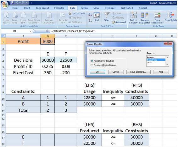
• A “Solver Results” box will appear. Select “Keep Solver Solution” and click “OK.”.

The solved worksheet is below.

Sensitivity Report

Written by Michael Chisholm and Doug Sutherland, Dec. 2009

Excel's solver program allows us to analyze how our profit would change if we had an alteration in our constraint values. These values can change due to a variety of reasons such as more readily available resources, technology advancements, natural disasters limiting resources, etc.

First, it analyzes whether the constraints are binding or non-binding. The binding constraints limit the profit output where the non-binding constraints do not limit the overall process. If the non-binding constraints were changed, the profit would not be effected as long the change in these constraints lies within the allowable increase and decrease that is indicated within the sensitivity report. If the binding constraints are changed, the profit will be directly affected. The affect on the profit is shown with shadow price values, also displayed in the sensitivity report. The shadow price is the resulting increase or decrease in profit per unit increase or decrease in the constraint. This applies as long as the change in constraint remains within the allowable increase or decrease where a linear relationship can be assumed.

The shadow price only analyzes the change in one variable at a time. In order to do two, you must plug the new constraint value for one of the variables and solve using solver. Using the new sensitivity report, analyze the effect that changing the second variable would have with the change being made in the first constraint.

Looking at Example 1 above, we will now walk through the steps on how to create a sensitivity report.

After clicking "solve" in excel, a solver results dialogue box appears as seen below.

There is a list of three options on the right; answer, sensitivity, and limits. Select the sensitivity option before clicking ok. A new tab will be generated in the worksheet titled "sensitivity 1." A view of the sensitivity report within the tab is seen below. As you can see, two tables are generated. For this example, resource A and product F are non-binding as shown with a shadow price of 0 and an infinite allowable increase. The allowable decrease is the amount the capacity changes until the final value is reached. Past this point the constraint would become a binding constraint. For the constraining variables (resource B and product E), their constraints are binding. Regarding resource B, if its constraint was increased by up to 5000 or decreased by up to 15000, this would have a linear effect on profit within this range. For each unit increase or decrease, the profit will change by 12 cents per unit, respectively. The same is true if our capacity for product E changes with it's allowable values and shadow price on the table.

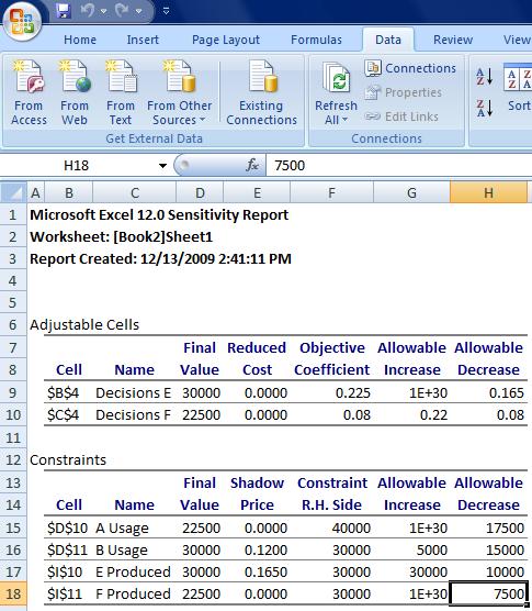
If the constraint on B increased by 5,000 lbs our new profit would be $8,600/day (8,000+.12*5,000). Instead, if our facility could increase production of E by 30,000 lb/day the resulting profit would be $12,950/day (8,000+.165*30,000).

Solving Linear Optimization Problems Using The Primal Simplex Algorithm

Written by: Tejas Kapadia and Dan Hassing [Note: needs specific reference, and also solution to the preceding problem by this method would be good -- R.Z.]

Instead of solving linear optimization problems using graphical or computer methods, we can also solve these problems using a process called the Primal Simplex Algorithm. The Primal Simplex Algorithm starts at a Basic Feasible Solution (BFS), which is a solution that lies on a vertex of the subspace contained by the constraints of the problem. In the Graph in Example 1, this subspace refers to the shaded region of the plot. Essentially, after determining an initial BFS, the Primal Simplex Algorithm moves through the boundaries from vertex to vertex until an optimal point is determined.

The basic procedure is the following:

1. Find a unit basis.
2. Set-up the problem in standard form using a canonical tableau.
3. Check optimality criterion.

1. If criterion passes, then stop, solution has been found.

4. Select an entering variable among the eligible variables.
5. Perform pivot step.
6. Go back to 1.

For simplicity, we will make the following assumptions:

1. The optimum lies on a vertex and is not unbounded on an extreme half-line.
2. The constraints are equations and not also inequalities.

1. In the case that the constraints are inequalities, slack variables will need to be introduced. Although the process is not very different in this case, we will ignore this to make the algorithm slightly less confusing.

3. Decision variables are required to be nonnegative.
4. The problem is a minimization problem. To turn a maximization problem into a minimization problem, multiply the objective function by -1 and follow the process to solve a minimization problem.

We will begin with the following example:

Objective Function: Minimize \(z=-x_{5}-8 x_{6}\)

Subject to the constraints:

\[\begin{align}
x_{1}-x_{5}+x_{6} &=2 \\[4pt]
x_{2}+x_{5}+x_{6} &=1 \\[4pt]
x_{3}+2 x_{5}+x_{6} &=5 \\[4pt]
x_{4}+x_{6} &=0 \\[4pt]
x_{i} &\geq 0
\end{align}\nonumber \]

First we begin by finding a unit basis:

A shortcut method to finding this unit basis is putting numbers in for each variable so that every constraint equation is satisfied.

In this case, setting , , and will satisfy the final equation and also set the values for , , and to 2, 1, and 5, respectively. Remember, these decision variables must be nonnegative.

Set up the canonical tableau in the following form:

As you can see, the first four rows correspond to the constraints, while the final row corresponds to the objective function. The “b” column corresponds to the right hand side (RHS) of the constraints. As you can see, the “-z” column is on the left hand side (LHS) of the equation, rather than the RHS.

First, we should perform pivot steps so that the tableau corresponds to the unit basis we found earlier. By performing pivot steps on , , , and , we will reach the feasible point where (, , , , , and ) = . Because , , and all equal zero, the pivot step on can actually be done on or , but in this example, we used . These pivot steps can be performed on any row as long as they are all different rows. In this example, we performed pivot steps on , , , using the Pivot and Gauss-Jordan Tool at people.hofstra.edu/Stefan_Waner/RealWorld/tutorialsf1/scriptpivot2.html. To use this tool, place the cursor on the cell that you wish to pivot on, and press “pivot”.

After four pivot steps, the tableau will look like this:

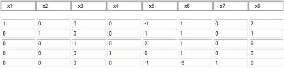
As you can see, this is identical to the initial tableau, as , , , and were set up such that an initial feasible point was already chosen.

The optimality criterion states that if the vector in the bottom left of the tableau is all positive, then an optimal solution exists in the “b” column vector, with the value at the bottom of the “b” column vector as the negative of the value of the objective function at that optimal solution. If this is not true, then a pivot step must be performed. In this example, clearly, a pivot step must be performed.

Next, we need to choose an entering variable. We want to choose an entering variable that has a negative element in the bottom row, meaning that the objective value could be improved if that variable was nonzero in the solution. So, we will choose in this example. Now, we must calculate ratios of each RHS coefficient divided by the coefficient of the entering variable in that row. In this case, the vector corresponding to this calculation would equal . We cannot pivot on a zero element, so we cannot pivot on the fourth row. We want to keep the RHS positive, so we cannot pivot on the first row. We must choose the minimum nonnegative ratio to remain at a feasible solution, so we choose the second row in the column, which has a ratio of 1/1.

After the pivot step:

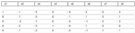
As we can see, has a negative coefficient in the bottom row, indicating the same step must be repeated on that column. We calculate ratios for that column, and get: . Consequently, we choose to pivot on the fourth row because it corresponds to the minimum nonnegative ratio of 0.

After another pivot step:

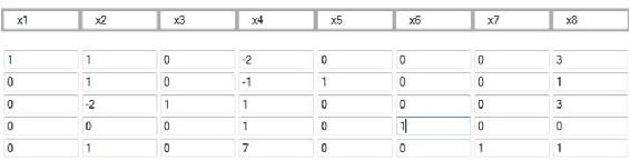
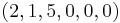
Because the bottom row is all positive, we are now at an optimal solution. To understand this final tableau, we look at each column for variables that only have one “1” in the column. If the column has only one “1”, the RHS value in that row is the value of that variable. In this case, , , and . Any variable that does not have just a single “1” in the column is equal to zero. So, the optimal solution is (, , , , , and ) = 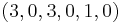, and the optimal value is (z was on the LHS in the tableau).

Now, we have successfully solved a linear optimization problem using the Primal Simplex Algorithm. Verification of the solution can be easily performed in Microsoft Excel.

References

1. D. E. Seborg, T. F. Edgar, D. A. Mellichamp: Process Dynamics and Control, 2nd Edition, John Wiley & Sons.
2. Rao, Singiresu S. Engineering Optimization - Theory and Practice, 3rd Edition, 129-135, John Wiley & Sons.