8.3: Non-linear Optimization

Last updated
Save as PDF

Page ID: 22410

Matthew Goh, Andrew King, & Edwin Yik
University of Michigan

$ \newcommand{\vecs}[1]{\overset { \scriptstyle \rightharpoonup} {\mathbf{#1}} } $

$ \newcommand{\vecd}[1]{\overset{-\!-\!\rightharpoonup}{\vphantom{a}\smash {#1}}} $

$ \newcommand{\id}{\mathrm{id}}$ $ \newcommand{\Span}{\mathrm{span}}$

( \newcommand{\kernel}{\mathrm{null}\,}\) $ \newcommand{\range}{\mathrm{range}\,}$

$ \newcommand{\RealPart}{\mathrm{Re}}$ $ \newcommand{\ImaginaryPart}{\mathrm{Im}}$

$ \newcommand{\Argument}{\mathrm{Arg}}$ $ \newcommand{\norm}[1]{\| #1 \|}$

$ \newcommand{\inner}[2]{\langle #1, #2 \rangle}$

$ \newcommand{\Span}{\mathrm{span}}$

$ \newcommand{\id}{\mathrm{id}}$

$ \newcommand{\Span}{\mathrm{span}}$

$ \newcommand{\kernel}{\mathrm{null}\,}$

$ \newcommand{\range}{\mathrm{range}\,}$

$ \newcommand{\RealPart}{\mathrm{Re}}$

$ \newcommand{\ImaginaryPart}{\mathrm{Im}}$

$ \newcommand{\Argument}{\mathrm{Arg}}$

$ \newcommand{\norm}[1]{\| #1 \|}$

$ \newcommand{\inner}[2]{\langle #1, #2 \rangle}$

$ \newcommand{\Span}{\mathrm{span}}$ $ \newcommand{\AA}{\unicode[.8,0]{x212B}}$

$ \newcommand{\vectorA}[1]{\vec{#1}} % arrow$

$ \newcommand{\vectorAt}[1]{\vec{\text{#1}}} % arrow$

$ \newcommand{\vectorB}[1]{\overset { \scriptstyle \rightharpoonup} {\mathbf{#1}} } $

$ \newcommand{\vectorC}[1]{\textbf{#1}} $

$ \newcommand{\vectorD}[1]{\overrightarrow{#1}} $

$ \newcommand{\vectorDt}[1]{\overrightarrow{\text{#1}}} $

$ \newcommand{\vectE}[1]{\overset{-\!-\!\rightharpoonup}{\vphantom{a}\smash{\mathbf {#1}}}} $

$ \newcommand{\vecs}[1]{\overset { \scriptstyle \rightharpoonup} {\mathbf{#1}} } $

$ \newcommand{\vecd}[1]{\overset{-\!-\!\rightharpoonup}{\vphantom{a}\smash {#1}}} $

$\newcommand{\avec}{\mathbf a}$ $\newcommand{\bvec}{\mathbf b}$ $\newcommand{\cvec}{\mathbf c}$ $\newcommand{\dvec}{\mathbf d}$ $\newcommand{\dtil}{\widetilde{\mathbf d}}$ $\newcommand{\evec}{\mathbf e}$ $\newcommand{\fvec}{\mathbf f}$ $\newcommand{\nvec}{\mathbf n}$ $\newcommand{\pvec}{\mathbf p}$ $\newcommand{\qvec}{\mathbf q}$ $\newcommand{\svec}{\mathbf s}$ $\newcommand{\tvec}{\mathbf t}$ $\newcommand{\uvec}{\mathbf u}$ $\newcommand{\vvec}{\mathbf v}$ $\newcommand{\wvec}{\mathbf w}$ $\newcommand{\xvec}{\mathbf x}$ $\newcommand{\yvec}{\mathbf y}$ $\newcommand{\zvec}{\mathbf z}$ $\newcommand{\rvec}{\mathbf r}$ $\newcommand{\mvec}{\mathbf m}$ $\newcommand{\zerovec}{\mathbf 0}$ $\newcommand{\onevec}{\mathbf 1}$ $\newcommand{\real}{\mathbb R}$ $\newcommand{\twovec}[2]{\left[\begin{array}{r}#1 \\ #2 \end{array}\right]}$ $\newcommand{\ctwovec}[2]{\left[\begin{array}{c}#1 \\ #2 \end{array}\right]}$ $\newcommand{\threevec}[3]{\left[\begin{array}{r}#1 \\ #2 \\ #3 \end{array}\right]}$ $\newcommand{\cthreevec}[3]{\left[\begin{array}{c}#1 \\ #2 \\ #3 \end{array}\right]}$ $\newcommand{\fourvec}[4]{\left[\begin{array}{r}#1 \\ #2 \\ #3 \\ #4 \end{array}\right]}$ $\newcommand{\cfourvec}[4]{\left[\begin{array}{c}#1 \\ #2 \\ #3 \\ #4 \end{array}\right]}$ $\newcommand{\fivevec}[5]{\left[\begin{array}{r}#1 \\ #2 \\ #3 \\ #4 \\ #5 \\ \end{array}\right]}$ $\newcommand{\cfivevec}[5]{\left[\begin{array}{c}#1 \\ #2 \\ #3 \\ #4 \\ #5 \\ \end{array}\right]}$ $\newcommand{\mattwo}[4]{\left[\begin{array}{rr}#1 \amp #2 \\ #3 \amp #4 \\ \end{array}\right]}$ $\newcommand{\laspan}[1]{\text{Span}\{#1\}}$ $\newcommand{\bcal}{\cal B}$ $\newcommand{\ccal}{\cal C}$ $\newcommand{\scal}{\cal S}$ $\newcommand{\wcal}{\cal W}$ $\newcommand{\ecal}{\cal E}$ $\newcommand{\coords}[2]{\left\{#1\right\}_{#2}}$ $\newcommand{\gray}[1]{\color{gray}{#1}}$ $\newcommand{\lgray}[1]{\color{lightgray}{#1}}$ $\newcommand{\rank}{\operatorname{rank}}$ $\newcommand{\row}{\text{Row}}$ $\newcommand{\col}{\text{Col}}$ $\renewcommand{\row}{\text{Row}}$ $\newcommand{\nul}{\text{Nul}}$ $\newcommand{\var}{\text{Var}}$ $\newcommand{\corr}{\text{corr}}$ $\newcommand{\len}[1]{\left|#1\right|}$ $\newcommand{\bbar}{\overline{\bvec}}$ $\newcommand{\bhat}{\widehat{\bvec}}$ $\newcommand{\bperp}{\bvec^\perp}$ $\newcommand{\xhat}{\widehat{\xvec}}$ $\newcommand{\vhat}{\widehat{\vvec}}$ $\newcommand{\uhat}{\widehat{\uvec}}$ $\newcommand{\what}{\widehat{\wvec}}$ $\newcommand{\Sighat}{\widehat{\Sigma}}$ $\newcommand{\lt}{<}$ $\newcommand{\gt}{>}$ $\newcommand{\amp}{&}$ $\definecolor{fillinmathshade}{gray}{0.9}$

Various conditions and situations are not adequately described using linear systems. In this case, nonlinear optimization may be applied. Unlike linear optimization, the optimal operating condition does not exist at the boundaries.

Quadratic Optimization

\[f(x)=c-x^{T} b+\frac{1}{2} x^{T} A x\nonumber \]

To optimize, it is necessary to find when the gradient of f is equal to zero.

\[\nabla f(x)=0\nonumber \]

\[\nabla f(x)=b-A x\nonumber \]

\[x_{*}=A^{-1} b\nonumber \]

It may be possible to solve the optimal quad x_* by a linear equation, approximated by a Taylor series.

\[f\left(x_{*}\right)=f(x)+\left(x_{*}-x\right)^{\prime} \nabla f(x)+\frac{1}{2}\left(x_{*}-x\right)^{\prime} \nabla \nabla f(x)\left(x_{*}-x\right)+\ldots\nonumber \]

Iterative Methods

When direct methods cannot solve the equation (i.e. A is not symmetric positive definite), iterative methods are possible [1].

By starting with an initial guess of quad x_i , an algorithm may lead to a $quad x_{i+1}$ that better satisfies the equation. Through iteration, theoretically, $quad x_\infty=x$ .

Applications

Finance: Portfolio optimization
Businesses: Optimize inventory
Engineering: Rigid body dynamics
Biochemistry: Kinetic modeling [2]

Example: Typical Nonlinear 3d Curves

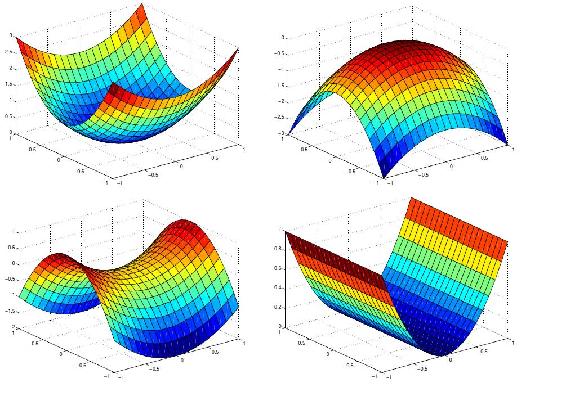
(Image from [1])

As observed, the optimal condition does not necessarily exist at the boundary of the curve.

Example: Quadratic Optimization

\[f(x)=\vec{c}^{T} \vec{x}+\frac{1}{2} \vec{x}^{T} Q \vec{x}\nonumber \]

where

\[\vec{c}^{T}=\left(c_{1}, c_{2}, \ldots, c_{n}\right)\nonumber \]

\[\vec{x}^{T}=\left(x_{1}, x_{2}, \ldots, x_{n}\right)\nonumber \]

For a quadratic system, $n=2$, thus, $Q$ (the quadratic term constant) is defined as a symmetric matrix as follows.

\[Q=\left[\begin{array}{ll}
Q_{1} & Q_{3} \\
Q_{3} & Q_{2}
\end{array}\right]\nonumber \]

Thus, multiplying out the $f$,

\[f(x)=\left(c_{1} x_{1}+c_{2} x_{2}\right)+\frac{1}{2}\left(Q_{1} x_{1}^{2}+2 Q_{3} x_{1} x_{2}+Q_{2} x_{2}^{2}\right)\nonumber \]

References

Lippert, Ross A. "Introduction to non-linear optimization." D.E. Shaw Research, February 25, 2008. http://www.mit.edu/~9.520/spring08/Classes/optlecture.pdf
Mendes, Pedro and Kell, Douglas B. "Non-linear optimization of biochemical pathways: application to metabolic engineering and parameter estimation." Journal of Bioinformatics, Volume 14, 869-883. 1998.
"Introduction to Non-linear optimization." Georgia Institute of Technology Systems Realization Laboratory. www.srl.gatech.edu/education/ME6103/NLP-intro.ppt

Search

Text Color

Text Size

Margin Size

Font Type