
9.5: PID tuning via Optimization
- Page ID
- 22416

Introduction
Tuning a controller is a method used to modify the effect a process change will have on the piece of equipment being controlled. The goal of tuning a system is to construct the most robust process possible. The method chosen for tuning a system varies depending on the parameter being measured, the sensitivity of the materials, the scale of the process, and many other variables unique to each process. This chapter discusses the basics of tuning a controller using predictive methods. To learn more about using an effect based method see the Classical Tuning section.
Optimization
When tuning a PID controller, constants \(K_{c}\), \(T_i\), and \(T_d\) need to be optimized. This can be accomplished using the following equation from the Classical Tuning section:
\[M V=K_{c}\left(e(t)+\frac{1}{T_{i}} \int_{0}^{t} e(\tau) d \tau+T_{d} \frac{d e(t)}{d t}\right) \label{1} \]
where
- \(MV\) is the manipulated variable (i.e. valve position) that the controller will change
- \(K_c\) accounts for the gain of the system
- \(T_i\) accounts for integrated error of the system
- \(T_d\) accounts for the derivative error of the system
Tuning by optimization uses computer modeling programs, such as Microsoft Excel, to find the optimal values for the coefficients \(K_c\), \(T_i\), and \(T_d\) to yield the minimum error (the Solver function in Excel can be used in this situation). For more information about the use of these parameters and their overall effects on the control system see the P, I, D, PI, PD, and PID control section.
Excel Modeling
For instructions on how to install Solver in Excel, see the Adding in the Solver Application in Excel 2007 section. For instruction on how to use Solver in Excel, see the Excel's Solver Tool section. Equation \ref{1} can be used in Excel to optimize the values of Kc, Ti, and Td. The following are the steps to optimize these constants:
- Pick a set point. Examples of set points include the temperature at which a reaction is expected to stay and the flow rate of a cooling stream.
- Make a column for error. Create a function in each cell so that the error is equal to the set point minus the actual value.
- Make a column that will calculate Equation 1.
- At the end of the error column, use the sum function to add up all of the errors in the column.
- Make three cells for Kc, Ti, and Td, and insert the initial values.
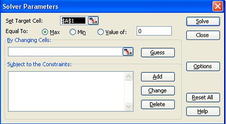
- Open the Solver function in Excel.
- In Solver, set the target cell to the summed errors cell. Set the target cell equal to the minimum value possible. Set the changing cells to Kc, Ti, and Td.
- Click 'Solve' to minimize the sum of the error and therefore optimize the Kc, Ti, and Td constants.
Tips for using Excel Solver to optimize PID controller parameters:
- When choosing initial values for your parameters, try starting with Kc=1, Ti=1000, and Td=1. Since Solver only does a limited number of iterations (usually set at 100), it may settle on an incorrect answer.
- Change the values for Kc manually and optimize with Solver until you get the lowest value in the target cell. This is the most efficient as Kc usually has the largest effect on a PID controller.
- Make sure to set constraints on your parameters in the 'Subject to the Constraints:' box in Solver (e.g. Kc > 0).
- Make sure you incorporate any physical limitations (e.g. maximum heater temperature) into your Excel model. Even though your system may not be close to the limit initially, Solver may try and go past that limit if it is not programmed into your model.
Industrial Application
The parameters (Kc, Ti, Td) found through optimization will not necessarily give the best control. To optimally tune a controller, a technician must adjust equipment to tune the process. So why is it necessary to tune by optimization? The parameters found by optimization give an accurate starting point for the technician.
Example of PID Tuning by Optimization
This example is based on the example in the CSTR Heat Exchange Model section. The goal is to optimize the PID controller for the coolant temperature. Follow the fully worked out example at: [Media:Optimal PID.xls Optimal PID]
As shown in the Excel file, the coolant temperature changes in response to variations from the set point by a PID type controller. Changing the Kc, Ti, and Td values using Solver, to minimize the total error, provided the values in the green box. On the second sheet, labeled 'disturbances', it can be seen that once optimized, the parameters should be fit to the system, regardless of changes in operating conditions.
It is important to note that the starting values you choose for the PID parameters will greatly affect your final results from using an excel solver. So you should always use your intuition to judge whether your starting values are reasonable or not. According to ExperTune , starting PID settings for common PID control loops are:
- Loop Type: Flow ; P = 50 to 100 ; I = 0.005 to 0.05 ; D = none ;
- Loop Type: Liquid Pressure ; P = 50 to 100 ; I = 0.005 to 0.05 ; D = none
- Loop Type: Gas Pressure ; P = 1 to 50 ; I = 0.005 to 0.05 ; D = 0.02 to 0.1 ;
- Loop Type: Liquid Level ; P = 1 to 50 ; I = 1 to 100 ; D = 0.01 to 0.05 ;
- Loop Type: Temperature ; P = 2 to 100 ; I = 0.2 to 50 ; D = 0.1 to 20 ;
The above values are rough, assume proper control loop design, ideal or series algorithm and do not apply to all controllers. These information should only be used as a possible consideration and should not be taken as an absolute starting value for all PID controls. For more information about the above values please go to www.expertune.com/tutor.html
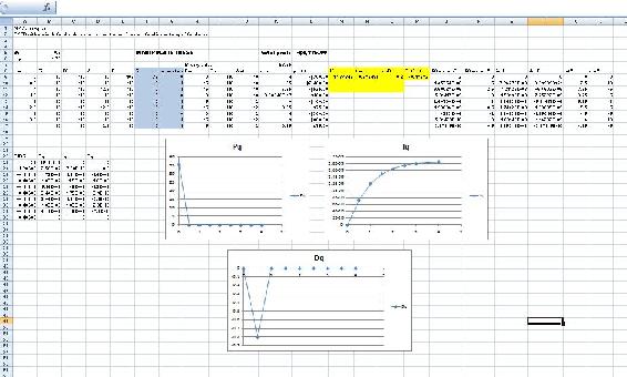
As mentioned before, to optimize the parameters in a PID-controlled system the solver function can be used in excel. However the solver function can sometimes run into its own problems because of the process it uses to solve for these “optimal” values. To ensure that solver gives you the correct optimal values, some manual “optimization” is needed. Using your excel sheet, the controller on the system can be separated into its different components P, I, and D. The behavior of each component can be monitored as the parameters are changed manually. Theoretically you would choose values that have every component reach steady-state over time. The excel solver can then be used as a precision tool. If your values are already closer to the optimal values, then solver should have no problem making them more precise. It is recommended that the graphs of the components be checked after using solver with your initial guesses. You may not have to go through this long and most of the time painful process. This is an example of how the P, I, and D plots change with different parameters. Note that the combined PID plot will also reach steady-state if each of the components reach steady-state.
(Parameters are not optimized) 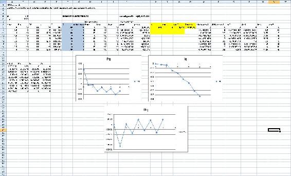
(Optimized parameters)
Example: Optimization of a Heat Exchanger
This example is based on the ODE Modeling in Excel of the Heat Exchange Model.
Find the best values of Kc, Ti, and Td in the given spreadsheet Media:PID_HeatExchange.xls.
Note the three different tabs:
- the first tab shows the problem to be solved
- the second is a step by step method for creating this sheet on your own
- the third is the answer to the problem
After using Solver:
- Click through the cells in one row to determine which parameters are affected by MV changes
- Change the values of Kc, Ti, and Td to see how they will effect the overall temperature profile. Which parameter has the greatest effect? Based on the equation, does this make sense?
What do you want to minimize when optimizing the constants Kc, Ti, and Td?
- Answer
-
time
References
- Svrcek, William Y., Mahoney, Donald P., Young, Brent R. "A Real Time Approach to Process Control", 2nd Edition. John Wiley & Sons, Ltd.
Contributor
- Authors: Andrew MacMillan, David Preston, Jessica Wolfe, Sandy Yu
- Stewards: YooNa Choi, Yuan Ma, Larry Mo, Julie Wesely