
9.6: PID Downsides and Solutions
- Page ID
- 22417

\( \newcommand{\vecs}[1]{\overset { \scriptstyle \rightharpoonup} {\mathbf{#1}} } \)
\( \newcommand{\vecd}[1]{\overset{-\!-\!\rightharpoonup}{\vphantom{a}\smash {#1}}} \)
\( \newcommand{\dsum}{\displaystyle\sum\limits} \)
\( \newcommand{\dint}{\displaystyle\int\limits} \)
\( \newcommand{\dlim}{\displaystyle\lim\limits} \)
\( \newcommand{\id}{\mathrm{id}}\) \( \newcommand{\Span}{\mathrm{span}}\)
( \newcommand{\kernel}{\mathrm{null}\,}\) \( \newcommand{\range}{\mathrm{range}\,}\)
\( \newcommand{\RealPart}{\mathrm{Re}}\) \( \newcommand{\ImaginaryPart}{\mathrm{Im}}\)
\( \newcommand{\Argument}{\mathrm{Arg}}\) \( \newcommand{\norm}[1]{\| #1 \|}\)
\( \newcommand{\inner}[2]{\langle #1, #2 \rangle}\)
\( \newcommand{\Span}{\mathrm{span}}\)
\( \newcommand{\id}{\mathrm{id}}\)
\( \newcommand{\Span}{\mathrm{span}}\)
\( \newcommand{\kernel}{\mathrm{null}\,}\)
\( \newcommand{\range}{\mathrm{range}\,}\)
\( \newcommand{\RealPart}{\mathrm{Re}}\)
\( \newcommand{\ImaginaryPart}{\mathrm{Im}}\)
\( \newcommand{\Argument}{\mathrm{Arg}}\)
\( \newcommand{\norm}[1]{\| #1 \|}\)
\( \newcommand{\inner}[2]{\langle #1, #2 \rangle}\)
\( \newcommand{\Span}{\mathrm{span}}\) \( \newcommand{\AA}{\unicode[.8,0]{x212B}}\)
\( \newcommand{\vectorA}[1]{\vec{#1}} % arrow\)
\( \newcommand{\vectorAt}[1]{\vec{\text{#1}}} % arrow\)
\( \newcommand{\vectorB}[1]{\overset { \scriptstyle \rightharpoonup} {\mathbf{#1}} } \)
\( \newcommand{\vectorC}[1]{\textbf{#1}} \)
\( \newcommand{\vectorD}[1]{\overrightarrow{#1}} \)
\( \newcommand{\vectorDt}[1]{\overrightarrow{\text{#1}}} \)
\( \newcommand{\vectE}[1]{\overset{-\!-\!\rightharpoonup}{\vphantom{a}\smash{\mathbf {#1}}}} \)
\( \newcommand{\vecs}[1]{\overset { \scriptstyle \rightharpoonup} {\mathbf{#1}} } \)
\(\newcommand{\longvect}{\overrightarrow}\)
\( \newcommand{\vecd}[1]{\overset{-\!-\!\rightharpoonup}{\vphantom{a}\smash {#1}}} \)
\(\newcommand{\avec}{\mathbf a}\) \(\newcommand{\bvec}{\mathbf b}\) \(\newcommand{\cvec}{\mathbf c}\) \(\newcommand{\dvec}{\mathbf d}\) \(\newcommand{\dtil}{\widetilde{\mathbf d}}\) \(\newcommand{\evec}{\mathbf e}\) \(\newcommand{\fvec}{\mathbf f}\) \(\newcommand{\nvec}{\mathbf n}\) \(\newcommand{\pvec}{\mathbf p}\) \(\newcommand{\qvec}{\mathbf q}\) \(\newcommand{\svec}{\mathbf s}\) \(\newcommand{\tvec}{\mathbf t}\) \(\newcommand{\uvec}{\mathbf u}\) \(\newcommand{\vvec}{\mathbf v}\) \(\newcommand{\wvec}{\mathbf w}\) \(\newcommand{\xvec}{\mathbf x}\) \(\newcommand{\yvec}{\mathbf y}\) \(\newcommand{\zvec}{\mathbf z}\) \(\newcommand{\rvec}{\mathbf r}\) \(\newcommand{\mvec}{\mathbf m}\) \(\newcommand{\zerovec}{\mathbf 0}\) \(\newcommand{\onevec}{\mathbf 1}\) \(\newcommand{\real}{\mathbb R}\) \(\newcommand{\twovec}[2]{\left[\begin{array}{r}#1 \\ #2 \end{array}\right]}\) \(\newcommand{\ctwovec}[2]{\left[\begin{array}{c}#1 \\ #2 \end{array}\right]}\) \(\newcommand{\threevec}[3]{\left[\begin{array}{r}#1 \\ #2 \\ #3 \end{array}\right]}\) \(\newcommand{\cthreevec}[3]{\left[\begin{array}{c}#1 \\ #2 \\ #3 \end{array}\right]}\) \(\newcommand{\fourvec}[4]{\left[\begin{array}{r}#1 \\ #2 \\ #3 \\ #4 \end{array}\right]}\) \(\newcommand{\cfourvec}[4]{\left[\begin{array}{c}#1 \\ #2 \\ #3 \\ #4 \end{array}\right]}\) \(\newcommand{\fivevec}[5]{\left[\begin{array}{r}#1 \\ #2 \\ #3 \\ #4 \\ #5 \\ \end{array}\right]}\) \(\newcommand{\cfivevec}[5]{\left[\begin{array}{c}#1 \\ #2 \\ #3 \\ #4 \\ #5 \\ \end{array}\right]}\) \(\newcommand{\mattwo}[4]{\left[\begin{array}{rr}#1 \amp #2 \\ #3 \amp #4 \\ \end{array}\right]}\) \(\newcommand{\laspan}[1]{\text{Span}\{#1\}}\) \(\newcommand{\bcal}{\cal B}\) \(\newcommand{\ccal}{\cal C}\) \(\newcommand{\scal}{\cal S}\) \(\newcommand{\wcal}{\cal W}\) \(\newcommand{\ecal}{\cal E}\) \(\newcommand{\coords}[2]{\left\{#1\right\}_{#2}}\) \(\newcommand{\gray}[1]{\color{gray}{#1}}\) \(\newcommand{\lgray}[1]{\color{lightgray}{#1}}\) \(\newcommand{\rank}{\operatorname{rank}}\) \(\newcommand{\row}{\text{Row}}\) \(\newcommand{\col}{\text{Col}}\) \(\renewcommand{\row}{\text{Row}}\) \(\newcommand{\nul}{\text{Nul}}\) \(\newcommand{\var}{\text{Var}}\) \(\newcommand{\corr}{\text{corr}}\) \(\newcommand{\len}[1]{\left|#1\right|}\) \(\newcommand{\bbar}{\overline{\bvec}}\) \(\newcommand{\bhat}{\widehat{\bvec}}\) \(\newcommand{\bperp}{\bvec^\perp}\) \(\newcommand{\xhat}{\widehat{\xvec}}\) \(\newcommand{\vhat}{\widehat{\vvec}}\) \(\newcommand{\uhat}{\widehat{\uvec}}\) \(\newcommand{\what}{\widehat{\wvec}}\) \(\newcommand{\Sighat}{\widehat{\Sigma}}\) \(\newcommand{\lt}{<}\) \(\newcommand{\gt}{>}\) \(\newcommand{\amp}{&}\) \(\definecolor{fillinmathshade}{gray}{0.9}\)Introduction
A proportional-integral-derivative (PID) controller is one of the most common algorithms used for control systems. It is widely used because the algorithm does not involve higher order mathematics, but still contains many variables. The amount of variables that are used allows the user to easily adjust the system to the desired settings. The algorithm for the PID uses a feedback loop to correct the difference between some measured value and the setpoint. It does this by calculating and outputting some action that will correct this error in the system. A PID controller has a proportional, integral and a derivative control which handles the current, past and predicted future of the signal error. For more information about PID, please refer to PID Intro. The PID controller can operate systems that run in a linear or nonlinear fashion. Tuning processes are done to the controller to tackle the possible nonlinear system. Limitations arise within the system because tuning is limited to only three different parameters (proportional, integral, and derivative controls). Additional information on tuning of PID can be found at [1] or [2]. The most common limitations that occur within the PID control specifically involve the integral control. The following article addresses some of the common limitations faced by each control type, with an emphasis on the integral control, and some solutions to overcome each of these limitations.
Proportional Control
The main purpose of the proportional control is minimize the fluctuations that occur within the system.
Limitations
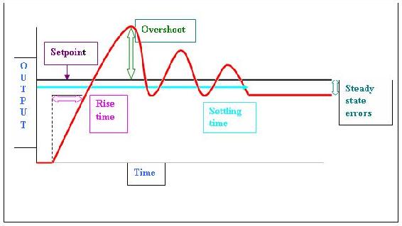
The P-controller usually has steady-state errors (the difference in set point and actual outcome) unless the control gain is large. As the control gain becomes larger, issues arise with the stability of the feedback loop. For instance, reducing the rise time implies a high proportional gain, and reducing overshoot and oscillations implies a small proportional gain. This is not possible to achieve in all systems.
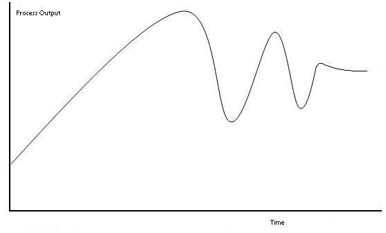
Below is a general process outcome diagram showing the terminology used above.
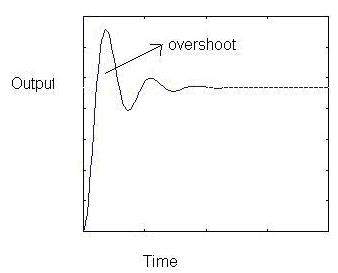
Below is a sample diagram of process output of proportional control.
Solutions
The way to eliminate these steady-state errors is by adding an integral action. The integral term in the equation drives the error to zero. Higher Integral constant (1 / Tt) drives the error to zero sooner but also invites oscillations and instability. Read on the integral control section below to know more about limitations associated with this integral term.
Below is a sample process output diagram when integral control is added.
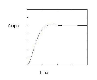
The above picture shows the reduction of overshoots and oscillations compared to the picture before adding the integral action.
Integral Control
The contribution from the integral term is proportional to both the magnitude of the error and the duration of the error. Summing the instantaneous error over time (integrating the error) gives the accumulated offset that should have been corrected previously. The accumulated error is then multiplied by the integral gain and added to the controller output. The magnitude of the contribution of the integral term to the overall control action is determined by the integral gain, \(K_i\).
The integral term is given by:
\[D_{\text {out }}=K_{d} \frac{d e}{d t} \nonumber \]
where
- Dout: is the Derivative output
- Kd: is the Derivative Gain, a tuning parameter
- e: is the Error = SP − PV
- t: is the Time or instantaneous time (the present)
Limitations
Windup
A basic knowledge of the concept of windup is useful before describing a specific type. Windup is defined as the situation when the feedback controller surpasses the saturation (i.e. maximum) limits of the system actuator and is not capable of instantly responding to the changes in the control error. The concept of the control variable reaching the actuator’s operation limits is reasonable considering the wide variety of operating conditions that are possible. When windup occurs the actuator constantly runs at its saturation limit despite any output the system might have. This means that the system now runs with an open loop instead of a constant feedback loop.
Integrator Windup
The most common type of windup that occurs is integrator windup. This occurs when the input into the system receives a sudden positive step command and causes a positive error when the system first responds to the actuator. If the rate of integration is larger than the actual speed of the system the integrator’s output may exceed the saturation limit of the actuator. The actuator will then operate at its limit no matter what the process outputs. The error will also continue to be integrated and the integrator will grow in size or “wind up”. When the system output finally reaches the desired value, the sign of the error reverses (e.g. y_{sp} " src="/@api/deki/files/18198/image-870.png">) and causes the integrator to “wind down” until things return back to normal. Through the wind down the control signal is still maximum for a long period of time and the response becomes delayed. The integrator takes a long period of time to fully recover to the operating range of the actuator. Integrator windup may occur from large set point changes, significant disturbances, or equipment malfunctions.
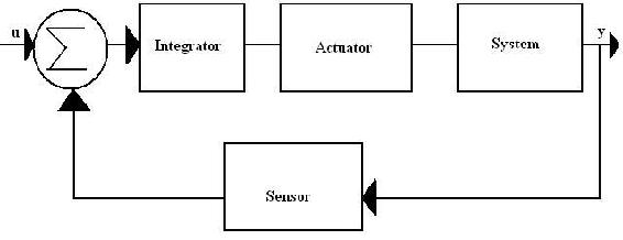
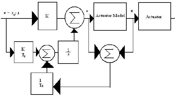
The illustration is a flowchart showing the specific steps that take place through the integrator controller. It shows the input ( ) and output of the system (
 ) , along with the integrator, the actuator, the system, and sensor involved in the process. The sigma used in each flowchart is used to represent the summation of all variables inputed to it.
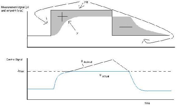
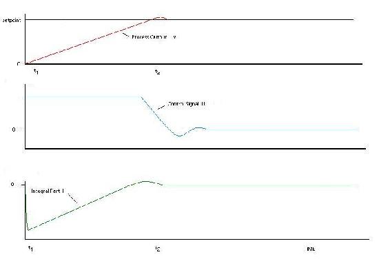
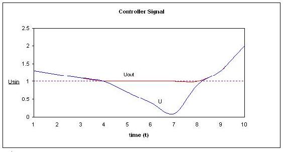
The graphs above are illustrations of integrator windup. The error ( ) is shown in the top graph as
  , where
  is the set point and is the measured signal. The bottom graph displays the control signal (). In this specific case of integrator windup, a set point change occurs and the control signal becomes saturated to its maximum amount
  . The system's error is still not eliminated though because the control signal is too small to make the error go to zero. In turn, this causes the integral to increase, which causes the desired control signal to increase. Therefore, there continues to be a difference between the desired control signal and the true control signal. After a period of time, the set point is lowered to a level where the controller is able to eliminate the control error. At this point
 y_{sp} " src="/@api/deki/files/18198/image-870.png">, which causes a change in the sign of the error. This change in sign causes the control signal to begin decreasing. The true signal (
 ) is stuck at for a while due to desired control signal u being above the limit . The changes in setpoints throughout this specific example occur because the input is changed in order to get a minimal error in the system.
File:Integrator windup output control integral5.JPG
The images above are another display of integrator windup. The top most shows the error, the middle shows the control signal, and the bottom shows the integral portion. The integral term begins to decrease, but remains positive, as soon as the error becomes negative at  . The output stays saturated due to the large integral termal that developes. The output signal remains at this level until the error becomes negative for a sufficiently long time (
 ). The control signal then fluctuates several times from its maxmimum to its minimum value and eventually settles down on a specific value. At every place where the control signal reaches its maximum the integral value has a large overshoot, and it follows that every place the control signal reaches a minimum the integral has a dampened oscillation. The integral term accounts for the removal of error in the oscillating system, which in turn causes the system's output to eventually reach a point that is so close to the setpoint that the actuator is no longer saturated. At this point, each graph begins to behave linearly and settles down. This example will be used later to show a solution to integral windup. The following section lists several ideas of how to prevent windup.
Solutions
The solutions involved in integral windup are termed as anti-windup schemes. Anti-windup is a method of counteracting the windup that happens in the integration that occurs in the integral controller of the PID.
Back-Calculation and Tracking
When the output is saturated, the integral term in the controller is recomputed so that it too is at the saturation limit. The integrator changes over time with the constant  . The difference between the output controller (
 ) and the actuator output () is found, and this is defined as an error signal. This error signal is then fed back to the input of the integrator with a gain of
  . The controller output is proportinal to the amount of time that the error is present. The error signal is only present when the actuator is saturated, therefore it will not have any effect on normal operation. With this method, the normal feedback path around process is broken and a new feedback path around the integrator is formed. The integrator input becomes:
\[\\frac {1}{T_t}e_s + \frac {K} {T_i}e \nonumber \]
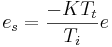
Knowing that  , the following equation can be made:
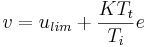
 is the control variable when saturated. The signs for and are always the same; therefore is always bigger than . This in turn prevents the windup in the integrator. The feedback gain is and is the rate at which the controller output is reset. is called the tracking time constant and is used to tune the amount of anti-windup. The flowchart shown below shows a PID controller with anti-windup implemented. The error signal in this process is only non-zero when the actuator is saturated. When this occurs the normal feedback path around the process is broken because the process input remains constant. A new feedback path is then formed around the integrator and causes the integrator output to be driven towards a value such that the integrator input becomes zero. Back-calculating never allows the input to the actuator to reach its actual saturation level because it forecasts what will actually go into the actuator model beforehand.
The following plots describe what happens to the same system (second example) described in the introduction to Integrator Windup section, only the controller now has anti-windup. The integrator output is at a value that causes the controller to be at the saturation limit, however, the integral is intially negative when the actuator is saturated (), which contrasts with the original behavior of the integrator. This has a positive effect on the process output, as it converges to the set point much quicker than the normal PI controller. There is only a slight overshoot in the process output ().
Conditional Integration
Conditional integration operates similarly to back-calculating. In this method the integration is turned off when the control is far from steady state. Integral action is then only used when certain conditions are met, otherwise the integral term is held constant. There are two possible conditions that may cause the integral to be set as a constant value. First, if the controller output is saturated (integration is shut off if error is positive but not negative), then the integrator input is set to a constant value. A second approach involves making the integrator constant when there is a large error. There is a disadvantage to the second approach because the controller may get stuck at a nonzero control error if the integral term has a large value at the time of switch off. For this reason, the first approach looks at the saturated controller output, not the saturated actuator output because referring to the actuator output will generate the same disadvantage[1] .
There is very little difference performance wise between integration and tracking, but they move the proportional bands differently. Read on to learn about proportional bands.
To demonstrate what it means to turn the integral term off, here is the equation (with logic) representing a control with conditional integration.
\[u(t)=K\left(e(t)+\frac{1}{T_{i}} \int e(t) d t\right)+u\left(t_{0}\right) \nonumber \]
If 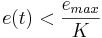 , then
Else 
Series Implementation
To avoid windup in an interacting controller a model of the saturation can be incorporated into the system. The model of saturation will limit the control signal indirectly. Too hard a limitation will cause an unnecessary limitation of the control action. Too weak a limitation will cause windup. More flexibility is provided if the saturation is positioned as follows:
With this setup it is possible to force the integral part to assume other preload values during saturation. The saturation function is replaced by the nonlinearity shown. This anti windup procedure is sometimes called a “batch unit” and is considered a type of conditional integration. It is mainly used for adjusting the overshoot during startup when there is a large set point change.
The Proportional Band
The proportional band is useful to understand when dealing with windup and anti windup schemes. The proportional band is a range such that if the instantaneous value of the process output or predicted value on the interval falls within the range, the actuator does not saturate. The proportional band (defined as the area between ylow,yhigh) is given by the following equations:
Control signal for PID control without derivative gain limitation:
\[\\ u = K*(b*y_{sp}) + I - K * T_d * \frac {dy}{dt} \nonumber \]
The predicted process output is given by
\[\\ y_p = y + T_d * \frac {dy}{dt} \nonumber \]
Combining the above equations for a maximum and minumum control signal ( and  )which corresponds to the points for which the actuator saturates,
\[\\ y_{low} = b * y_{sp} + \frac {I - u_{max}}{K} \nonumber \]
\[\\ y_{high} = b * y_{sp} + \frac {I - u_{min}}{K} \nonumber \]
If the predicted output is in the proportional band, the controller operates linearly. The control signal saturates when the predicted output is outside of the proportional band. The following plot illustrates how the proportional band is useful in understanding windup for the same example. At time equals zero, the proportional band is increased, indicating that the integral part is increasing. Immediately after , the output is greater that the setpoint, which causes the integral part to start to decrease. As can be seen, the output value, does not reach the proportional band until it is greater than the setpoint, . When the output finally reaches the proportional band at , it goes through the band very quickly, due to the band changing at a high rate. The control signal decreases immediately and saturates in the opposite direction, causing the output to decrease and approach the setpoint. This process repeats as the output value converges with the setpoint.
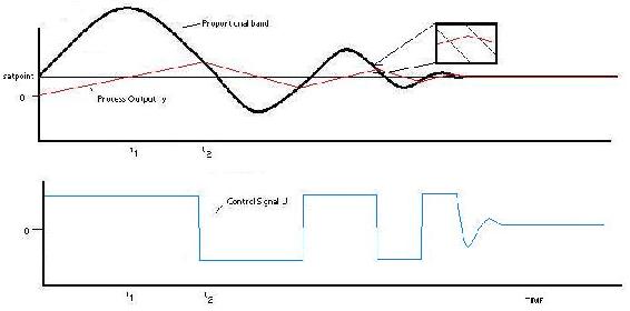
The tracking time constant has a major influence on the proportional band. The proportional band is moved closer to the output because of tracking. The tracking time constant determines the rate that the proportional band moves at.
Real Life Scenario
Imagine a situation where a water storage tank that is needed to store water and supply for use in a plant and it is necessary to keep the water level constant. A level sensor is installed to keep track of the water level in the tank, and it sends this data to the controller. The controller has a set point for instance 75% full. The rate of water entering the tank is increased by opening valve and decreased by closing the valve. In the case of integral windup, the valve is all the way closed or open and the actuator sends the signal to close it more or open it more which is not possible.
Derivative Control
Derivative action can be thought of as making smaller and smaller changes as one gets close to the right value, and then stopping in the correct region, rather than making further changes. Derivative control quantifies the need to apply more change by linking the amount of change applied to the rate of change needed. For example, an accelerator would be applied more as the speed of the car continues to drop. However, the actual speed drop is independent of this process. On its own, derivative control is not sufficient to restore the speed to a specific value. Pairing the match in change with a proportionality constant is enough to properly control the speed.
The derivative control is usually used in conjunction with P and/or I controls because it generally is not effective by itself. The derivative control alone does not know where the setpoint is located and is only used to increase precision within the system. This is only control type that is open loop control (also known as feedforward loop). The derivative control operates in order to determine what will happen to the process in the future by examining the rate of change of error within the system. When the derivative control is implemented the following general equation is used:
\[u(t)=\frac{1}{T_{d}} \frac{d}{d t} e(t)+u\left(t_{0}\right) \nonumber \]
where
 = control signal
 = derivative time
 = error
 = initial control signal
This equation shows the derivative control is proportional to the change in error within the system.
Limitations of Derivative Control
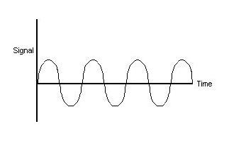
The major problem associated with this control is the noise problem. When the frequency within the system is high (change in error of the system is large), taking the derivative of this signal may amplify the signal greatly. Therefore, small amounts of noise within the system will then cause the output of system to change by a great amount. In these circumstances, it is often sensible use a PI controller or set the derivative action of a PID controller to zero.
The following is a graphical represenation of some sinusoidal output signal function of a system.
Solutions
To eliminate/minimize this problem, an electronic signal filter can be included in the loop. Electronic signal filters are electronic circuits which perform signal processing functions, specifically intended to remove unwanted signal components and/or enhance wanted ones. Electronic filters can be: passive or active, analog or digital, discrete-time (sampled) or continuous-time, linear or non-linear, etc. The most common types of electronic filters are linear filters, regardless of other aspects of their design.
For more information on electronic signal filters, reference the following website:
en.Wikipedia.org/wiki/Electronic_filter
The derivative term in the equation is usually changed by putting a first order filter on the term so that the derivative does not amplify the high frequency noise that is attenuated. Below is a sample outcome figure of a possible derivative of the output signal shown above along with the filtered signal.
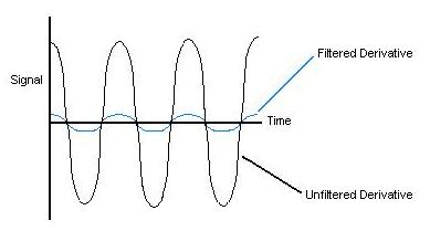
As shown, it is possible for the amplitude to be magnified when the derivative is taken for a sinusoidal function. A filter is usually a set of complicated equations that are added to the derivative that effect the function as shown.
Robustness of PID controllers
When designing a PID controller it is important to not only create a controller that will correct the error in an efficient manor, but also a robust controller. No matter how good the controller is if it cannot handle the magnitude of certain disturbances then it will not be able to perform well and complete the job. The robustness of a controller is the ability of the controller to withstand disturbances and still operate effectively. In order to calculate controller robustness, a weighted sum of the integral of the squared controller effort (ISC) and the integral of the squared controller error (ISE) is calculated. The smaller the weighted sum the more robust the controller.
ISE = 0 ∫ ∞ e(t)2 dt
ISC = 0 ∫ ∞ [u(∞)-u(t)]2 dt
IT = w ISC + ISE
In these equations u is the input variable, w is the weight factor which is based on downstream processes and IT is the total error and controller effort. The weight factor is used to assign a higher significance to the ISC or the ISE. The significance depends on the design and whether it is more important to have minimal error and tight control or less controller effort with more error. Low values of w are used when tight control is desired. Robustness calculations are determined experimentally. The robustness depends a lot on the type of control used, whether it is feedback, feed- forward, cascade, or a combination.
Notes on robustness
It is important to realize that when calculating the robustness of a feed forward system, the system will reach a steady state, but it is unlikely that the system will reach the original set point. As a result, the feed forward system will most likely be less robust than a feedback system. The reason the feed-forward system doesn't return to the set point but finds a new steady state is because it uses open loop control and there are no sensors to inform it that its adjustment to the disturbance did not work correctly. For this reason, feed-forward controllers are sometimes coupled with a feedback system. When combined the feed-forward controller can now see if its corrections achieved the desired result or not, resulting in a more robust controller.
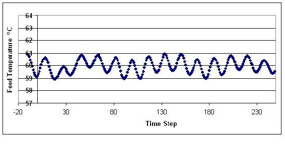
Example Robustness Calculation
In this system, the controller is regulating the temperature of the feed to a certain downstream process. After collecting experimental data from your controller, the following graph was made.
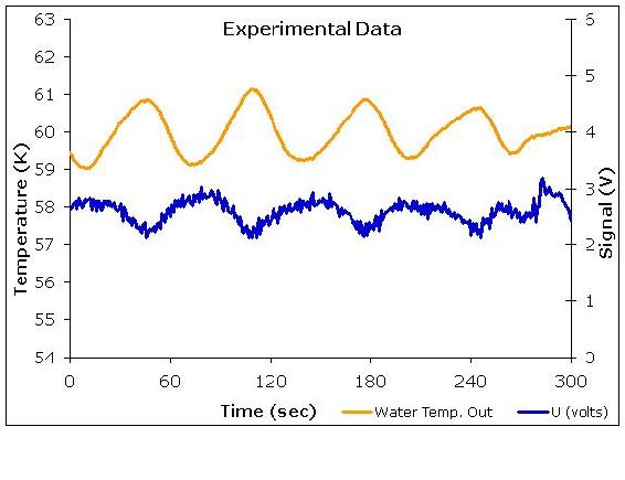
Using this graph the squared controller effort and the squared error can also be graphed and the ISE and ISC can be calculated. The graph of the corresponding effort and error can be seen below.
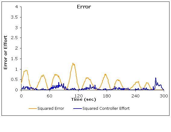
Using the squared controller effort and the squared error graph, the robustness can be calculated. To find the integral of the squared error and the squared controller effort the trapezoid rule can be used.
\[IT = w ISC + ISE \nonumber \]
\[ISC= 21 ISE =94 \nonumber \]
Assuming a weight factor of 1, the robustness of the controller is 115.
Consider the below output from using one of the controllers. The general equation of the output signal, U = K(e). What problems do you see in the below picture and how can you correct them?
Solution
The response time is very high, and it has a high overshoot and oscillation problems as well as steady-state errors. The equation confirms that it is a P-controller and
A heat exchanger uses a PID control system to control the temperature of the outlet of tube side of the heat exchanger. It’s required to keep water at 20 C for the cooling of an effluent from an exothermic reaction. The specific controller has a min output of 1 volt and a max output of 6 volts. The experimental data shows a large lag time in the controller’s ability to cool the incoming fluid (the lower portion of the sinusoidal curve). The following data shows the correlation between the controller output and the calculated signal. Describe the type of problem and a possible solution to the problem.
Solution
The Problem shown is an example of integrator-windup. The controllers calculated signal is lower than the min output that it can handle. This explains the lag time seen for the lower portion of the sinusoidal curve. To fix this problem the integral control can be recomputed using back track calculation.
(a) You are using a PID controller to maintain the feed to a reactor at a constant temperature. It is imperative that the feed remain within 1 °C of the set-point. You’ve tuned your PID control system according to the Ziegler-Nichols open loop system and obtained the following values for Kc, τI, and τD: Kc = 0.218, 1/τI = 0.0536, τD = 4.67
You want to know if these are good control values or if they can be improved. Your control variable output looks like this:
Additionally, you have available the following plot of the voltage output from your control parameters:
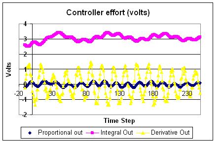
Is this system in control? If so, explain why. If not, explain why and what (qualitative) improvements to the PID gains will bring the system into better control.
Solution
The system is in control in that it appears to roughly stay within the defined acceptable boundaries of ±1°C. However, it does display oscillation, indicating that the system is working a little harder than maybe it has to. Looking at the controller voltage output, we see that the derivative gain is giving high oscillations. Thus maybe decreasing this gain would keep the system in control with a little less wear and tear on the control valves.
(b) At another flow rate, you observe the following behavior in your controller:
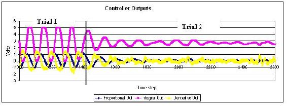
Is the system under control in Trial 1? In Trial 2? Why or why not? What physically happened between trials to give the observed change in output?
Solution: In trial 1, without even looking at the direct system output, we can guess that it is probably not in control. The controller output voltage indicates that the integral gain is way too high, and its wild oscillations will doubtlessly be causing oscillations in the system. Physically, this means that the system is opening and closing the valve constantly, creating a lot of wear and tear on the machinery, and probably overcompensating for small changes and further destabilizing the system. In trial 2, we can see that the integral voltage oscillations have damped, indicating that the gain has been reduced. As these oscillations level out, the oscillations in the other control gains also damp down, as the system comes into better control and none of the terms are working as hard as they had been before.
Note this is an open-ended problem meant to give readers an intuition about PID controllers
Imagine the classic differential equation problem of two tanks in a series governed by the differential equations:
\[\frac{d h_{1}}{d t}=P I D-K_{1} \sqrt{h_{1}} \nonumber \]
\[\frac{d h_{2}}{d t}=K_{1} \sqrt{h_{1}}-K_{2} \sqrt{h_{2}} \nonumber \]
\[\P I D=1+K_{p} e(t)+\frac{1}{t_{i}} \int_{0}^{t} e(\tau) d \tau+t_{d} \frac{d e(t)}{d t}]
where
- h1 = height of tank 1
- h2 = height of tank 2
- Ki = valve constant associated to tank 1 or 2
The valve constants K1 = 5 and K2 = 5 and the set point is 3. What values of Kp, ti, and td will cause the two tanks to reach steady state the fastest? Also what values will give the most oscillations?
Solution
Click on this link for the worked out Mathematica solution
Other questions that can be explored with slight modifications of the code are:
1. Will the values of Kp, ti, and td yield similar results if the PID controller was placed on tank 2? What new values of Kp, ti, and td will cause the two tanks to reach steady state the fastest?
2. For the values of Kp, ti, and td that causes the two tanks o reach steady state the fastest, what happens if you increase K1? What will happen if you increase K2?
Label the following general response charts as overdamped, critically damped, underdamped, undamped, and unstable.
(a) 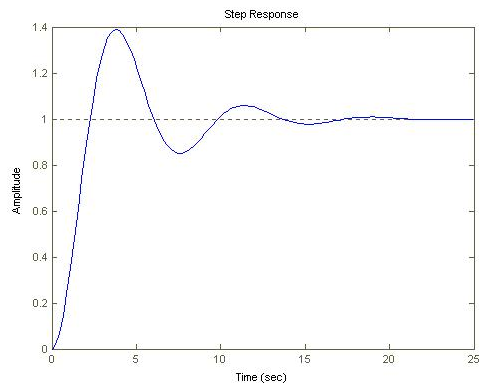
(b) 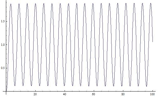
(c) 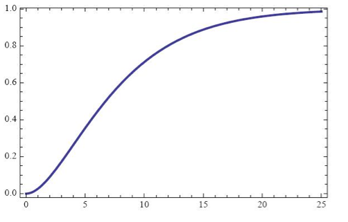
(d) 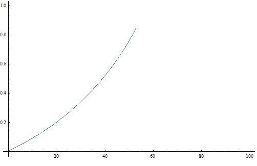
(e) 
Answers
a)Underdamped b)Undamped c)Critically Damped d)Unstable e)Overdamped
What is a back-calculation used for?
- To reduce noise problems
- To reduce steady-state errors
- To reduce errors in integral term
- To reduce errors in proportional term
What is a proportional band?
- A way to eliminate errors in integral term
- A way to eliminate errors in proportional term
- A way to eliminate errors in derivative term
- A way to understand anti-windup problem
References
- Bhattacharyya, Shankar P., Datta & Silva, PID Controllers for Time-Delay Systems, 2005 [1]
- Astrom, Karl J., Hagglund, Tore., Advanced PID Control, ISA, The Instrumentation, Systems and Automation Society.
- U of Texas chE
- Wikipedia Article, PID Controller, en.Wikipedia.org/wiki/PID_control
Contributors
- Authors: Ashwini Miryala, Kyle Scarlett, Zachary Zell, Brandon Kountz
- Stewards: Brian Hickner, Lennard Gan, Addison Heather, Monique Hutcherson