
10.2: Linearizing ODEs
- Page ID
- 22500

\( \newcommand{\vecs}[1]{\overset { \scriptstyle \rightharpoonup} {\mathbf{#1}} } \)
\( \newcommand{\vecd}[1]{\overset{-\!-\!\rightharpoonup}{\vphantom{a}\smash {#1}}} \)
\( \newcommand{\dsum}{\displaystyle\sum\limits} \)
\( \newcommand{\dint}{\displaystyle\int\limits} \)
\( \newcommand{\dlim}{\displaystyle\lim\limits} \)
\( \newcommand{\id}{\mathrm{id}}\) \( \newcommand{\Span}{\mathrm{span}}\)
( \newcommand{\kernel}{\mathrm{null}\,}\) \( \newcommand{\range}{\mathrm{range}\,}\)
\( \newcommand{\RealPart}{\mathrm{Re}}\) \( \newcommand{\ImaginaryPart}{\mathrm{Im}}\)
\( \newcommand{\Argument}{\mathrm{Arg}}\) \( \newcommand{\norm}[1]{\| #1 \|}\)
\( \newcommand{\inner}[2]{\langle #1, #2 \rangle}\)
\( \newcommand{\Span}{\mathrm{span}}\)
\( \newcommand{\id}{\mathrm{id}}\)
\( \newcommand{\Span}{\mathrm{span}}\)
\( \newcommand{\kernel}{\mathrm{null}\,}\)
\( \newcommand{\range}{\mathrm{range}\,}\)
\( \newcommand{\RealPart}{\mathrm{Re}}\)
\( \newcommand{\ImaginaryPart}{\mathrm{Im}}\)
\( \newcommand{\Argument}{\mathrm{Arg}}\)
\( \newcommand{\norm}[1]{\| #1 \|}\)
\( \newcommand{\inner}[2]{\langle #1, #2 \rangle}\)
\( \newcommand{\Span}{\mathrm{span}}\) \( \newcommand{\AA}{\unicode[.8,0]{x212B}}\)
\( \newcommand{\vectorA}[1]{\vec{#1}} % arrow\)
\( \newcommand{\vectorAt}[1]{\vec{\text{#1}}} % arrow\)
\( \newcommand{\vectorB}[1]{\overset { \scriptstyle \rightharpoonup} {\mathbf{#1}} } \)
\( \newcommand{\vectorC}[1]{\textbf{#1}} \)
\( \newcommand{\vectorD}[1]{\overrightarrow{#1}} \)
\( \newcommand{\vectorDt}[1]{\overrightarrow{\text{#1}}} \)
\( \newcommand{\vectE}[1]{\overset{-\!-\!\rightharpoonup}{\vphantom{a}\smash{\mathbf {#1}}}} \)
\( \newcommand{\vecs}[1]{\overset { \scriptstyle \rightharpoonup} {\mathbf{#1}} } \)
\(\newcommand{\longvect}{\overrightarrow}\)
\( \newcommand{\vecd}[1]{\overset{-\!-\!\rightharpoonup}{\vphantom{a}\smash {#1}}} \)
\(\newcommand{\avec}{\mathbf a}\) \(\newcommand{\bvec}{\mathbf b}\) \(\newcommand{\cvec}{\mathbf c}\) \(\newcommand{\dvec}{\mathbf d}\) \(\newcommand{\dtil}{\widetilde{\mathbf d}}\) \(\newcommand{\evec}{\mathbf e}\) \(\newcommand{\fvec}{\mathbf f}\) \(\newcommand{\nvec}{\mathbf n}\) \(\newcommand{\pvec}{\mathbf p}\) \(\newcommand{\qvec}{\mathbf q}\) \(\newcommand{\svec}{\mathbf s}\) \(\newcommand{\tvec}{\mathbf t}\) \(\newcommand{\uvec}{\mathbf u}\) \(\newcommand{\vvec}{\mathbf v}\) \(\newcommand{\wvec}{\mathbf w}\) \(\newcommand{\xvec}{\mathbf x}\) \(\newcommand{\yvec}{\mathbf y}\) \(\newcommand{\zvec}{\mathbf z}\) \(\newcommand{\rvec}{\mathbf r}\) \(\newcommand{\mvec}{\mathbf m}\) \(\newcommand{\zerovec}{\mathbf 0}\) \(\newcommand{\onevec}{\mathbf 1}\) \(\newcommand{\real}{\mathbb R}\) \(\newcommand{\twovec}[2]{\left[\begin{array}{r}#1 \\ #2 \end{array}\right]}\) \(\newcommand{\ctwovec}[2]{\left[\begin{array}{c}#1 \\ #2 \end{array}\right]}\) \(\newcommand{\threevec}[3]{\left[\begin{array}{r}#1 \\ #2 \\ #3 \end{array}\right]}\) \(\newcommand{\cthreevec}[3]{\left[\begin{array}{c}#1 \\ #2 \\ #3 \end{array}\right]}\) \(\newcommand{\fourvec}[4]{\left[\begin{array}{r}#1 \\ #2 \\ #3 \\ #4 \end{array}\right]}\) \(\newcommand{\cfourvec}[4]{\left[\begin{array}{c}#1 \\ #2 \\ #3 \\ #4 \end{array}\right]}\) \(\newcommand{\fivevec}[5]{\left[\begin{array}{r}#1 \\ #2 \\ #3 \\ #4 \\ #5 \\ \end{array}\right]}\) \(\newcommand{\cfivevec}[5]{\left[\begin{array}{c}#1 \\ #2 \\ #3 \\ #4 \\ #5 \\ \end{array}\right]}\) \(\newcommand{\mattwo}[4]{\left[\begin{array}{rr}#1 \amp #2 \\ #3 \amp #4 \\ \end{array}\right]}\) \(\newcommand{\laspan}[1]{\text{Span}\{#1\}}\) \(\newcommand{\bcal}{\cal B}\) \(\newcommand{\ccal}{\cal C}\) \(\newcommand{\scal}{\cal S}\) \(\newcommand{\wcal}{\cal W}\) \(\newcommand{\ecal}{\cal E}\) \(\newcommand{\coords}[2]{\left\{#1\right\}_{#2}}\) \(\newcommand{\gray}[1]{\color{gray}{#1}}\) \(\newcommand{\lgray}[1]{\color{lightgray}{#1}}\) \(\newcommand{\rank}{\operatorname{rank}}\) \(\newcommand{\row}{\text{Row}}\) \(\newcommand{\col}{\text{Col}}\) \(\renewcommand{\row}{\text{Row}}\) \(\newcommand{\nul}{\text{Nul}}\) \(\newcommand{\var}{\text{Var}}\) \(\newcommand{\corr}{\text{corr}}\) \(\newcommand{\len}[1]{\left|#1\right|}\) \(\newcommand{\bbar}{\overline{\bvec}}\) \(\newcommand{\bhat}{\widehat{\bvec}}\) \(\newcommand{\bperp}{\bvec^\perp}\) \(\newcommand{\xhat}{\widehat{\xvec}}\) \(\newcommand{\vhat}{\widehat{\vvec}}\) \(\newcommand{\uhat}{\widehat{\uvec}}\) \(\newcommand{\what}{\widehat{\wvec}}\) \(\newcommand{\Sighat}{\widehat{\Sigma}}\) \(\newcommand{\lt}{<}\) \(\newcommand{\gt}{>}\) \(\newcommand{\amp}{&}\) \(\definecolor{fillinmathshade}{gray}{0.9}\)Introduction
Chemical engineering processes often operate in nonlinear and unsteady manners (i.e. not always at steady state), and are generally governed by nonlinear ordinary differential equations (ODEs). The ODE is a relation that contains functions of only one independent variable and derivatives with respect to that variable. Many studies have been devoted to developing solutions to these equations, and in cases where the ODE is linear it can be solved easily using an analytical method. However, if the ODE is nonlinear and not all of the operating parameters are available, it is frequently difficult or impossible to solve equations directly. Even when all the parameters are known, powerful computational and mathematical tools are needed to completely solve the ODEs in order to model the process. In order to simplify this modeling procedure and obtain approximate functions to describe the process, engineers often linearize the ODEs and employ matrix math to solve the linearized equations.
A linear equation is an equation in which each term is either a constant or the product of a constant times the first power of a variable. These equations are called "linear" because they represent straight lines in Cartesian coordinates. A common form of a linear equation in the two variables \(x\) and \(y\) is \(y = mx + b\). This is opposed to a nonlinear equation, such as
\[m = e^x + x^2 + 2x + 5. \nonumber \]
Even though \(2x + 5\) is a linear portion of the equation, \(e^x\) and \(x^2\) are not. Any nonlinear terms in an equation makes the whole system nonlinear.
Non-linear system of equations:
\[\begin{align*}
\dfrac{d A}{d t} &=3 A^{2}+2 B+C-7 D^{3} \\[4pt]
\dfrac{d B}{d t}&=A+C^{2}+2 D \\[4pt]
\dfrac{d C}{d t}&=A+4 B^{2}-C^{2} \\[4pt]
\dfrac{d D}{d t}&=2 C-D \end{align*} \nonumber \]
After linearization (around the steady state point {-0.47,-0.35,0.11,0.23}:
\[\left(\begin{array}{c}
A^{\prime} \\
B^{\prime} \\
C^{\prime} \\
D^{\prime}
\end{array}\right)=\left(\begin{array}{cccc}
-2.83 & 2 & 1 & 0 \\
1 & 0 & 0.23 & 0 \\
1 & -2.78 & -0.23 & 0 \\
0 & 0 & 2 & 0
\end{array}\right)\left(\begin{array}{c}
A \\
B \\
C \\
D
\end{array}\right)+\left(\begin{array}{c}
k_{1} \\
k_{2} \\
k_{3} \\
k_{4}
\end{array}\right) \nonumber \]
Note that each equation is comprised solely of first order variables.
Even though it is unlikely that the chemical engineering process to be modeled operates in a linear manner, all systems can be approximated as linear at a point. This is preferred as linear systems are much easier to work with than nonlinear equations. Although linearization is not an exact solution to ODEs, it does allow engineers to observe the behavior of a process. For example, linearized ODEs are often used to indicate exactly how far from steady state a given process deviates over specified operating ranges. This wiki page discusses how to solve a linearized ODE by hand and by using Mathematica, and proceeds to work out several examples of linearized ODEs commonly seen in chemical engineering practice.
Applications to Chemical Engineering
As mentioned above, linearizing ODEs allows engineers to understand the behavior of their system at a given point. This is very important because many ODEs are impossible to solve analytically. It will also lead to determining the local stability of that point. Most of the time a system will be linearized around steady state, but this is not always the case. You may be interested in understanding the behavior of your system at its operating point or equilibrium state (not necessarily steady state). The linearization approach can be used for any type of nonlinear system; however, as a chemical engineer, linearizing will usually involve ODEs. Chemical engineers use ODEs in applications such as CSTRs, heat exchangers, or biological cell growth.
It is also important to understand the advantages and disadvantages of linearizing a system of ODEs:
Advantages
- Provides a simpler, more convenient way to solve the ODEs
- The behavior of a process can be observed
- Any type or order of ODE can be used
Disadvantages
- The solution is only an exact solution at the chosen point; otherwise it is an approximation and becomes less accurate away from the point
- Although linearizing is a quicker alternative, it takes time to initially learn the process (ex: using Mathematica)
Another use for linearization of the equations that govern chemical processes is to determine the stability and characteristics of the steady states. Systems of linearized ODEs can be used to do this, and the methods of doing so can be found in Fixed Points, Eigenvectors and Eigenvalues, and Using eigenvalues and eigenvectors to find stability and solve ODEs
General Procedure for Linearization
Linearization is the process in which a nonlinear system is converted into a simpler linear system. This is performed due to the fact that linear systems are typically easier to work with than nonlinear systems. For this course, the linearization process can be performed using Mathematica. The specific instructions on how to do this can be found below.
- Choose a relevant point for linear approximation, two options available are:
- Steady state- points where system does not change
- Current location- given where you are now
- Calculate the Jacobian matrix at that point. The Jacobian is essentially a Taylor series expansion.
- Solve to find unknown constants using algebraic methods.
Linearization by Hand
In order to linearize an ordinary differential equation (ODE), the following procedure can be employed. A simple differential equation is used to demonstrate how to implement this procedure, but it should be noted that any type or order of ODE can be linearized using this procedure.
1. Use a Taylor series expansion (truncating after the linear terms) to approximate the right-hand side of the ODE.
Let’s say we start with the following ODE:
\[\frac{d x}{d t}=f(x)=3 x^{2}.\nonumber \]
This ODE describes the behavior of some variable, \(x\), with respect to time.
A Taylor series is a series expansion of a function about a point. If \(x= a\), an expansion of a real function is given by:
\[f(x)=\sum_{n=0}^{\infty} \frac{f^{n}(a)}{n !}(x-a)^{n}\nonumber \]
\[f(x) = f(a)+f^{\prime}(a)(x-a)+\frac{f^{2}(a)}{2 !}(x-a)^{2}+\frac{f^{3}(a)}{3 !}(x-a)^{3}-\ldots+\frac{f^{n}(a)}{n !}(x-a)^{n}+\ldots\nonumber \]
When \(x=0\), the function is also known as Maclaurin series. Taylor’s theorem states that any function satisfying certain conditions can be expressed as a Taylor series.
For simplicity’s sake, only the first two terms (the zero- and first-order) terms of this series are used in Taylor approximations for linearizing ODEs. Additionally, this truncation (ie. "chopping" off the \(n=2\) and higher terms from the polynomial shown above) assures that the Taylor Series is a linear polynomial. If more terms are used, the polynomial would have \((x − a)^2\) and higher order terms and become a nonlinear equation. The variable ‘\(a\)’ in the Taylor series is the point chosen to linearize the function around. Because it is desired that most processes run at steady state, this point will be the steady state point. So, our differential equation can be approximated as:
\[\frac{d x}{d t}=f(x) \approx f(a)+f^{\prime}(a)(x-a)=f(a)+6 a(x-a)\nonumber \]
Since \(a\) is our steady state point, \(f(a)\) should always be equal to zero, and this simplifies our expression further down to:
\[\frac{d x}{d t}=f(x) \approx f^{\prime}(a)(x-a)=6 a(x-a)\nonumber \]
The graph shown above shows the approximation of f(x) at (x,f(x)). As mentioned previously, linearization is only an approximation for any given function near a continuous point. When working with a system of ODEs, the Jacobian is written as a matrix. It is the matrix of constants needed to describe a system's linearity. The Jacobian may be thought of as how much a system is distorted to take on a linear identity. A Jacobian matrix will always be a square(#rows = #columns) and it shows how each equation varies with each variable. The Jacobian matrix is defined as:
\[J\left(x_{1}, \ldots, x_{n}\right)=\left[\begin{array}{ccc}
\frac{\partial y_{1}}{\partial x_{1}} & \cdots & \frac{\partial y_{1}}{\partial x_{n}} \\
\vdots & \ddots & \vdots \\
\frac{\partial y_{n}}{\partial x_{1}} & \cdots & \frac{\partial y_{n}}{\partial x_{n}}
\end{array}\right]\nonumber \]
And is used as such for this non-linear set of equations
\[\begin{array}{l}
\frac{d x}{d t}=2 x^{2}+\cos (5 y)-12 \arctan (z-3) \\
\frac{d y}{d t}=7 y^{3}+\sin (5 x) \\
\frac{d z}{d t}=1.3 \log (x+y)
\end{array}\nonumber \]
The linearized system is
\[\left[\begin{array}{l}
x^{\prime} \\
y^{\prime} \\
z^{\prime}
\end{array}\right]=\left[\begin{array}{lll}
J_{1} & J_{2} & J_{3} \\
J_{4} & J_{5} & J_{6} \\
J_{7} & J_{8} & J_{9}
\end{array}\right]\left[\begin{array}{l}
x \\
y \\
z
\end{array}\right]+\left[\begin{array}{l}
c_{1} \\
c_{2} \\
c_{3}
\end{array}\right]\nonumber \]
The square matrix is the Jacobian.
Lets say you have the following set of equations and you want to find its Jacobian matrix around the point \(A=3,\,B=2).
\[\frac{d A}{d t}=3 A-A^{2}-A B\nonumber \]
\[\frac{d B}{d t}=6 B-A B-2 B^{2}\nonumber \]
We find the Jacobian by taking the derivative of each equation with respect to each variable.
\[\frac{d\left(3 A-A^{2}-A B\right)}{d A}=3-2 A-B\nonumber \]
\[\frac{d\left(3 A-A^{2}-A B\right)}{d B}=-A\nonumber \]
\[\frac{d\left(6 B-A B-2 B^{2}\right)}{d A}=-B\nonumber \]
\[\frac{d\left(6 B-A B-2 B^{2}\right)}{d B}=6-A-4 B\nonumber \]
These are the equations in the matrix. The values of the variables from whatever point we are linearizing are then put into these equations and calculated out to get the Jacobian.
\[J a c=\left[\begin{array}{cc}
3-2 A-B & -A \\
-B & 6-A-4 B
\end{array}\right] A=4, B=2\nonumber \]
\[J a c=\left[\begin{array}{ll}
-7 & -4 \\
-2 & -6
\end{array}\right]\nonumber \]
2. Change the approximation by linearizing around a steady state point in order to describe how the process deviates from steady state.
The following substitution can be made:
\[\frac{d x}{d t}=\frac{d(x-a)}{d t}\nonumber \]
\[\frac{d(x-a)}{d t} \approx 6 a(x-a)\nonumber \]
This substitution is allowed because ‘a’ is a constant, and the derivative of a constant is zero.
Substituting (x-a) for x signifies that our differential equation now shows how our function, x, deviates away from the steady state value, a, with respect to time. This deviation, (x-a), is commonly expressed as x′. It should also be noted that the quantity ‘6a’ is a constant, and thus will be further recognized as ‘A’.
Our final linearized equation becomes:
\[\frac{d x^{\prime}}{d t} \approx A x^{\prime}\nonumber \]
The once nonlinear ODE,
\[\frac{d x}{d t}=f(x)=3 x^{2}\nonumber \]
has now been simplified into a linear differential equation.
The procedure of linearization typically occurs around the steady state point or points of a specified process. Engineers anticipate a certain change in output for the particular steady state point, and may proceed to linearize around it to complete their approximation. Please follow the graphic below for further detail. Note that a steady state point occurs when \(dx / dt = 0\)
\[\rror Plot Color New 1.jpg\nonumber \]
As can be seen, moving farther away from the steady state point results in significantly larger deviation, and thus error (actual-linearization).
Occasionally, for very unique operating conditions, plant management may decide to momentarily run a process outside of strict steady state conditions (perhaps a unique start-up procedure, shut-down recovery, etc.). To reinforce the concept of linearization around an unsteady state point (arbitrarily chosen in this example), please consider the following visual representation. Note that a=50 and C=7500 in the first plot.
\[\ew Image 2.jpg\nonumber \]
The second plot is a magnification of a small section of the first plot. As one can readily notice, both the linear approximation and the actual graph overlap almost exactly over this small range. This illustrates how this particular linearization could be used to approximate this region of the function and can describe its behavior quite accurately. This approximating technique using the linearization of ODE can be performed around different points (different values of a) using the same method in order to model the behavior of the rest of the dx/dt vs x function. Note: frequent recalculation of the integration constant, C, permits for increased accuracy in approximation.
Example of a Simple Linearization Process in Use
Provided a circumstance in which developing a rigorous analytical solution is unfeasible due to time, access to computing resources, or mathematical ability, the linearization process offers a convenient and swift alternative.
An appropriate introduction to linearization application is featured in section 5.3 of the Bequette reading and has been described below.
The following model describes the behavior of tank height as a function of time (t), faced with a steady- state incoming liquid flowrate. dh/dt represents the change in height of the fluid contained within the tank as a function of time, h indicates the height (or level) or the fluid contained within the tank, F represents the magnitude of incoming flow. The following model describes the tank level/height fluctuation as function of both the current height (h) and flow (F). Fluid enters the tank as flow per area of the inlet(F/A), and leaves as a function of a corrective proportional term, β, also per area of the outlet, multiplied by the square root of the current height.
Instead of fluid leaving through this term, we may also consider it a form of feedback control, which subsequently reduces the amount of inlet fluid instead ( depends on the application, the final result is identical). Therefore:
\[\frac{d h}{d t}=f(h, F)=\frac{F}{A}-\frac{\beta}{A} * \sqrt{h} \nonumber \]
Important note about the relevance of the provided variables:
Fs indicates the initial flow rate for the described system and is important in calculating the intercept and subsequently the calculative corrective term for the linearization (if the linearization is not performed at steady-state, as in this example). hs describes the tank height for the specified flow rate, Fs. Upon plugging in the value of hs into the linearized formula, you will notice that f(h,Fs) = 0, the point on the plot where both the linearization and the characteristic equation coincide (i.e. are tangent).
h remains a variable for the derivation so that students may notice that it is a dependant variable (dependent upon the flowrate). Bequette must (and does) provide both the values for Fs, hs so that a linearization may proceed (otherwise we will simply have an equation describing the slope with no characteristic point to pass through).
System Parameters (Fs is an example flow rate at steady state, this information is used to determine the intercept of the linearized formula):
\[A=1 f t^{2} ; h_{s}=5 f t ; \beta=\frac{1}{\sqrt{5}} \frac{f t^{2.5}}{m i n} ; F_{s}=\frac{1 f t^{3}}{m i n} \nonumber \]
Rewriting the system with the input variables:
\[\frac{d h}{d t}=f\left(h, F_{s}\right)=1+\frac{1}{\sqrt{5}} * \sqrt{h} \nonumber \]
To linearize around a certain point, simply evaluate the derivative of the desired function and add in a corrective constant, C, represented by the value of the function at the initial (specified) condition.
\[\(h,F_s) \approx f(h,F_s)+ \frac{\partial{f}}{\partial{h}}|_h, _{F_s}(h-h_s) \nonumber \]
\[\(h,F_s) \approx 0+ \frac{-1}
Callstack:
    at (Bookshelves/Industrial_and_Systems_Engineering/Chemical_Process_Dynamics_and_Controls_(Woolf)/10:_Dynamical_Systems_Analysis/10.02:_Linearizing_ODEs), /content/body/div[5]/p[15]/span, line 1, column 2
Selecting, h=5 to linearize around, we present an adapted version of the text example (linearization is in red):
\[\(h,1) \approx 0+ \frac{-1}
Callstack:
    at (Bookshelves/Industrial_and_Systems_Engineering/Chemical_Process_Dynamics_and_Controls_(Woolf)/10:_Dynamical_Systems_Analysis/10.02:_Linearizing_ODEs), /content/body/div[5]/p[17]/span, line 1, column 2
\[\(5,1) \approx 0+ \frac{-1}
Callstack:
    at (Bookshelves/Industrial_and_Systems_Engineering/Chemical_Process_Dynamics_and_Controls_(Woolf)/10:_Dynamical_Systems_Analysis/10.02:_Linearizing_ODEs), /content/body/div[5]/p[18]/span, line 1, column 2
f(h,1)approx. = − 0.1 * (h − 5)
\[\isual 3.jpg \nonumber \]
The physical significance of this example:
The model describes a situation where a tank maintains the steady state set point, a level (height) of 5 feet, by regulating the input (and/or output) flow rate(s). A height above the preferred level of 5 ft. results in a negative height change per time; conversely, a height below the preferred level of 5 ft. results in a positive height change per time, so as to always approach the steady state level.
Also, please note that the linearized system responds relatively slower than the characteristic equation system (non- linear)when tank level falls below 5 ft. and faster than the characteristic equation system when the tank level is above 5 ft.
Please read on below to learn a step-by-step technique on how to complete this method for most equations.
Linearization using Mathematica
Most ODEs are not as simple as the example worked out above. For those that can be solved analytically, the 'by-hand' method from the previous section can be used, although the math becomes tricky and tedious when one is dealing with systems of ODEs. For those that cannot be solved analytically and can only be approximated numerically, it is sometimes impossible to do the numerical analysis by hand. For these ODEs, powerful computational tools such as Mathematica can be used to perform linearization.
The following Mathematica file contains a worked out example (CSTR w/ heat exchange). This example contains multiple ODEs and multiple types of variables. When dealing with ODEs, there are three main type of variables: state, input, and output. State variables describes the system at any given time (ie. Ca, Cb, T, etc.). Input variables are simply inputs into the system. Output variables are those that are not directly related to the inputs, but are dependent on the state variables (ie. k, the reaction constant). You will discover in the CSTR example that it is necessary to linearize state variables and output variables separately.
Before proceeding to the Mathematica file we will first present some of the Mathematica commands that will be necessary to linearize the CSTR example.
Note that you need to press shift+enter (shift+return on Mac) after a command to evaluate the expression.
Example:
In[1]= ((0.04587*54.32497+4.59058433734947^7)/48700043)^131.94564
Out[1]= 0.000411241
Another thing to note is the use of assignment and equality operators.
= is called immediate assignment operator and := is called delayed assignment operator. When immediate assignment operator is used, the right hand side of the operator is evaluated every time an assignment is made. However, when delayed assignment operator is used, the right hand side is evaluated only when the value of the expression on the left hand side is requested.
lhs=rhs rhs is intended to be the "final value" of lhs (e.g., f[x_]=1-x^2) lhs:=rhs rhs gives a "command" or "program" to be executed whenever you ask for the value of lhs (e.g., f[x_]:=Expand[1-x^2])
p := x^3 - 6 x^2 + 11 x - 6
This input, which produces no output, assigns the polynomial expression to the variable p. The assignment is done because this polynomial may be used again later, so the assignment saves retyping it. The equality operator ==, which is used here to form the equation we are asking Mathematica to solve:
In[2]:= Solve[p == 0]
Out[2]=
Callstack:
    at (Bookshelves/Industrial_and_Systems_Engineering/Chemical_Process_Dynamics_and_Controls_(Woolf)/10:_Dynamical_Systems_Analysis/10.02:_Linearizing_ODEs), /content/body/div[6]/p[14]/span, line 1, column 4
When solving nonlinear ODEs using Mathematica, it is necessary to form a matrix and there are several commands that can be used to create matrices.
D[X,Y]
This command takes the partial derivative of an expression (X) with respect to a variable (Y) defined by the user. The first term in the square brackets is the experession you wish to differentiate, the second is the variable you wish to differentiate with respect to.
AppendRows[column1,column2]
This command creates a matrix by combining two columns. In order to use this command you must first load the Matrix Manipulation package using the command <<LinearAlgebra`MatrixManipulation`
M = Callstack:
at (Bookshelves/Industrial_and_Systems_Engineering/Chemical_Process_Dynamics_and_Controls_(Woolf)/10:_Dynamical_Systems_Analysis/10.02:_Linearizing_ODEs), /content/body/div[6]/p[20]/b/span, line 1, column 3
This command creates a matrix, in this case a 3x3 matrix.
MatrixForm[X]
This command displays a specified matrix in matrix form.
These commands will allow us to proceed with the linearization of the CSTR problem shown below. 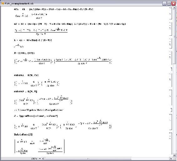
The first three commands input the equations that govern the behavior of the concentration, Ca, the temperature, T, and the rate of reaction, k. Once the equations have been entered into Mathematica a matrix, M, with one column and two rows containing the equations for Ca and T is created. Next two new matrices are created by taking the derivative of matrix M is with respect to both Ca and T. These matrices, called column1 and column2 respectively, together form the Jacobian of the system and is then displayed in matrix form. The Jacobian matrix is the matrix of all first-order partial derivatives of a vector-valued function. Its importance lies in the fact that it represents the best linear approximation to a differentiable function near a given point. For example, given a set y=f(x) of n equations in variables x1, x2,...,xn, the Jacobian matrix is defined as following:
\[\acobianmatrix.gif \nonumber \]
\[\athematicapg2.JPG \nonumber \]
Now that we have the Jacobian we need to create a matrix containing the deviation from steady state for each of the variables. This matrix, SS, contains the actual concentration and temperature, C and T, minus the steady state concentration and temperature, Cas and Ts. The matrix is then displayed in matrix form. We now have both the Jacobian and the deviation matrix for the state variables. The next four commands create the Jacobian and deviation matrix for the output variable, k. The first command creates the Jacobian matrix by taking the derivative of the k equation with respect to Ca and T. The Jacobian is then shown in matrix form. Finally the deviation matrix for k is created in the same manner as above and then displayed in matrix form. Note that because k is defined above, this expression is substituted in for k in the deviation matrix. The following Mathematica file contains the code shown above with extra comments explaining why each step is performed Media:cstr_example.nb. It may be useful to downolad this file and run the program in Mathematica yourself to get a feel for the syntax. Downloading the file will also allow you to make any changes and edits to customize this example to another example of interest.
Note: This file needs to be saved to your computer, and then opened using Mathematica to properly run.
To see another example lets linearize the first 4 differential equations given in the introduction section.
Non-linear system of equations:
\[\frac{dA}{dt}=3A^2+2B+C-7D^3 \nonumber \]
\[\frac{dB}{dt}=A+C^2+2D \nonumber \]
\[\frac{dC}{dt}=A+4B^2-C^2 \nonumber \]
\[\frac{dD}{dt}=2C-D \nonumber \]
After linearization (around the steady state point {-0.47,-0.35,0.11,0.23}:
\[\left(\begin{array}{c}
A^{\prime} \\
B^{\prime} \\
C^{\prime} \\
D^{\prime}
\end{array}\right)=\left(\begin{array}{cccc}
-2.83 & 2 & 1 & -1.10 \\
1 & 0 & 0.23 & 2 \\
1 & -2.78 & -0.23 & 0 \\
0 & 0 & 2 & -1
\end{array}\right)\left(\begin{array}{l}
A \\
B \\
C \\
D
\end{array}\right)+\left(\begin{array}{c}
0.50 \\
0.01 \\
0.47 \\
0
\end{array}\right) \nonumber \]
The 4 differential equations above are added into a Mathematica code as “eqns” and “s1” is the fixed points of the differentials. The steady state values found for “a, b, c, and d” are called "s1doubleBrackets(7)” After the steady state values are found, the Jacobian matrix can be found at those values.
To find “k1, k2, k3, and k4” the constants of the Linearization matrix equation, “m1” must be defined, which is the 2nd matrix on the right-hand side of the Linearization matrix equation.
To determine the k values (in matrix form), execute the dot product of "m1" and the “Jac” matrix, which is done by the "." operator. Therefore it should look like "Jac.m1"
To obtain the k values, determing the "Jac.m1" at the steady state values, which is done by the "/." operator. Therefore it should look like “Jac.m1/.s1doubleBrackets(7)”
Let's say you have a system governed by the following system of equations:
\[\begin{align*} \dfrac{d X_{a}}{d t} &=3 X_{a}^{2}+2 X_{b}+F_{o} \\[4pt] \dfrac{d X_{b}}{d t} &=6 X_{a}+9 X_{b}^{2}+X_{a} X_{b}+F_{o} \\[4pt] Y &=X_{a}^{2}+3 * F_{o}^{2} \end{align*} \nonumber \]
In this case, \(X_a\) and \(X_b\) are state variables (they describe the state of the system at any given time), \(F_o\) is an input variable (it enters the system and is independent of all of the state variables), and \(Y\) is the output of the system and is dependent on both the state and input variables. Please linearize this system using Mathematica.
Use the Mathematica file presented in the article to linearize the CSTR example presented in the ODE & Excel CSTR model with heat exchangewiki around the steady state (T = 368.4K and Ca = 6.3mol/L). Use the constants presented in their example. Use the linearization to approximate Ca at 369K.
Solution
The linear approximation gives concentration of a (Ca) of 7.13 mol/L. The Mathematica file used to solve this problem can be downloaded here. Media:LinearizationExample.nb If you are having trouble running the Mathematica file try right clicking the link and using the Save Target As option.
In an ODE linearization, what point in the process is the linearization generally centered around?
a. Starting point
b. Ending point
c. Steady-state point
d. Half-way point
- Answer
-
Answer: c
What does the D[] function in Mathematica do?
a. Find the determinant of a matrix
b. Finds the partial derivative a function or functions
c. Find the dot product of two matrices
d. Integrate a matrix or function
- Answer
-
Answer: b
References
- Bequette, B. Wayne. Process Dynamics: Modeling, Analysis, and Simulation. Prentice- Hall PTR, Upper Saddle River, NJ 07458 (c) 2006.
- Kravaris, Costas. Chemical Process Control: A Time Domain Approach, Appendix A. Department of Chemical Engineering, University of Michigan, Ann Arbor, MI.
- Bhatti, M. Asghar. Practical Optimization Methods With Mathematica Applications. Springer Telos.