10.4: Using Eigenvalues and Eigenvectors to Find Stability and Solve ODEs

Introduction

Eigenvalues and eigenvectors are very useful in the modeling of chemical processes. When designing the controls for a process it is necessary to create a program to operate these controls. Differential equations are used in these programs to operate the controls based on variables in the system. These equations can either be solved by hand or by using a computer program. The solutions for these differential equations will determine the stability of the system. After finding this stability, you can show whether the system will be stable and damped, unstable and undamped (so that there is constant fluctuation in the system), or as an unstable system in which the amplitude of the fluctuation is always increasing. For the first case, a stable and damped system, if there is a change, the system will adjust itself properly to return to steady state. For the other two cases, the system will not be able to return to steady state. For the undamped situation, the constant fluctuation will be hard on the system and can lead to equipment failure. The final situation, with the ever increasing amplitude of the fluctuations will lead to a catastrophic failure.

There are a couple ways to develop the differential equation used to determine stability. First, you can create a differential equation to guide the system where the variables are the readings from the sensors in the system. A second method would be using actual data found from running the system. You could fit a differential equation to this data and use that equation for stability determination.

In this section on Eigenvalue Stability, we will first show how to use eigenvalues to solve a system of linear ODEs. Next, we will use the eigenvalues to show us the stability of the system. After that, another method of determining stability, the Routh stability test, will be introduced. For the Routh stability test, calculating the eigenvalues is unnecessary which is a benefit since sometimes that is difficult. Finally, the advantages and disadvantages of using eigenvalues to evaluate a system's stability will be discussed.

Solving ODEs

Eigenvalues and eigenvectors can be used as a method for solving linear systems of ordinary differential equations (ODEs). The method is rather straight-forward and not too tedious for smaller systems. See The Eigenvector Eigenvalue Method for solving systems by hand and Linearizing ODEs for a linear algebra/Jacobian matrix review. When trying to solve large systems of ODEs however, it is usually best to use some sort of mathematical computer program. Mathematica is a program that can be used to solve systems of ordinary differential equations when doing them by hand is simply too tedious. Once one overcomes the syntax of Mathematica, solving enormous systems of ordinary linear differential equations becomes a piece of cake!

Using Eigenvalues to Solve a System

A linear system will be solve by hand and using Eigenvalues[ ] expression in Mathematica simultaneously. Note that, in the Mathematica inputs below, "In[]:=" is not literally typed into the program, only what is after it. The syntax needed to be typed is the line following "In[]=" . The term is used here to more accurately demonstrate coding in Mathematica. To find a general solution of the linear system of ordinary differential equation:

\[\frac{d x}{d t}=4 x+8 y \nonumber \]

\[\frac{d y}{d t}=10 x+2 y \nonumber \]

We first put the system in matrix form:

\[A=\left[\begin{array}{l}
\frac{d x}{d t} \\
\frac{d y}{d t}
\end{array}\right]=\left[\begin{array}{cc}
4 & 8 \\
10 & 2
\end{array}\right]\left[\begin{array}{l}
x \\
y
\end{array}\right] \nonumber \]

Where we can see that

\[A=\left[\begin{array}{cc}
4 & 8 \\
10 & 2
\end{array}\right] \nonumber \]

In mathematica, we can use the following code to represent A:

In[1]:= MatrixForm [{{4,8},{10,2}}]
Out[1]:=

The eigenvalues λ₁ and λ₂, are found using the characteristic equation of the matrix A, det(A- λI)=0.

Therefore, λ₁ = 12 and λ₂ = − 6

We can use Mathematica to find the eigenvalues using the following code:

In[2]:= Eigenvalues[{{4,8},{10,2}}]

Out[2]:={12,-6}

Now, for each eigenvalue (λ₁=12 and λ₂=-6), an eigenvector associated with it can be found using , where is an eigenvector such that

i) For λ₁=12

This will lead to the equations (1) &(2):

(1)

(2)

The Mathematica input is:

In[3]:= eqn1= -8x+8y==0
In[4]:= eqn2= 10x-10y==0

In[5]:= Solve[{eqn1,eqn2},{x,y}]

Out[5]:=
Equations (1) & (2) lead to the solution

ii) For λ₂=-6,

This will lead to the equations (3) & (4):

(3)

(4)

The Mathematica input is:

In[6]:= eqn3= 10x+8y==0
In[7]:= eqn4= 10x+8y==0

In[8]:= Solve[{eqn3,eqn4},{x,y}]

Out[8]:=

Equations (3) & (4) lead to the solution .

Recall that the direction of a vector such as is the same as the vector or any other scalar multiple. Therefore, to get the eigenvector, we are free to choose for either the value x or y.

i) For λ₁ = 12
We have arrived at y = x. As mentioned earlier, we have a degree of freedom to choose for either x or y. Let’s assume that x=1. Then, y=1 and the eigenvector associated with the eigenvalue λ₁ is

ii) For λ₂ = − 6
We have arrived at . Let’s assume that x = 4. Then, y = -5 and the eigenvector associated with the eigenvalue λ₂ is .

These two eigenvalues and associated eigenvectors yield the solution:

\[\left[\begin{array}{l}
x(t) \\
y(t)
\end{array}\right]=c_{1}\left[\begin{array}{l}
1 \\
1
\end{array}\right] e^{12 t}+c_{2}\left[\begin{array}{c}
4 \\
-5
\end{array}\right] e^{-6 t} \nonumber \]

Hence a general solution of the linear system in scalar form is:

\[\begin{align*}{l} x(t)&=c_{1} e^{12 t}+c_{2} 4 e^{-6 t} \\[4pt] y(t)&=c_{1} e^{12 t}-c_{2} 5 e^{-6 t} \end{align*} \nonumber \]

Solving a System Using DSolve

Using the same linear system of ordinary differential equations:

\[\frac{d x}{d t}=4 x+8 y \nonumber \]

\[\frac{d y}{d t}=10 x+2 y \nonumber \]

We input the differential equations to Mathematica with the following command:

In:= ODEs={x'[t]==4x[t]+8y[t],y'[t]==10x[t]+2y[t]}

where x'[t] = and y'[t] =

After entering the equations, we use the DSolve function:

In:= DSolve[ODEs, {x[t], y[t]}, t]

Mathematica will output the solution:

Out:=

ParseError: invalid DekiScript (click for details)

Callstack:
    at (Bookshelves/Industrial_and_Systems_Engineering/Chemical_Process_Dynamics_and_Controls_(Woolf)/10:_Dynamical_Systems_Analysis/10.04:_Using_eigenvalues_and_eigenvectors_to_find_stability_and_solve_ODEs), /content/body/div[2]/div[2]/p[10]/span, line 1, column 1

This set of equations, although looks more complicated than the first one, is actually the same.

Stability

Eigenvalues can be used to determine whether a fixed point (also known as an equilibrium point) is stable or unstable. A stable fixed point is such that a system can be initially disturbed around its fixed point yet eventually return to its original location and remain there. A fixed point is unstable if it is not stable. To illustrate this concept, imagine a round ball in between two hills. If left alone, the ball will not move, and thus its position is considered a fixed point. If we were to disturb the ball by pushing it a little bit up the hill, the ball will roll back to its original position in between the two hills. This is a stable fixed point. Now image that the ball is at the peak of one of the hills. If left undisturbed, the ball will still remain at the peak, so this is also considered a fixed point. However, a disturbance in any direction will cause the ball to roll away from the top of the hill. The top of the hill is considered an unstable fixed point.

The eigenvalues of a system linearized around a fixed point can determine the stability behavior of a system around the fixed point. The particular stability behavior depends upon the existence of real and imaginary components of the eigenvalues, along with the signs of the real components and the distinctness of their values. We will examine each of the possible cases below.

Imaginary (or Complex) Eigenvalues

When eigenvalues are of the form \(a+bi\), where \(a\)and \(b\) are real scalars and \(i\) is the imaginary number \(\sqrt{-1}\), there are three important cases. These three cases are when the real part is positive, negative, and zero. In all cases, when the complex part of an eigenvalue is non-zero, the system will be oscillatory.

Positive Real Part

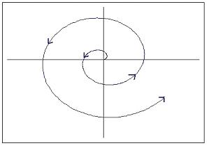
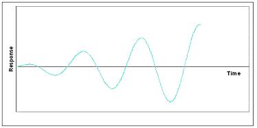
When the real part is positive, the system is unstable and behaves as an unstable oscillator. This can be visualized as a vector tracing a spiral away from the fixed point. The plot of response with time of this situation would look sinusoidal with ever-increasing amplitude, as shown below.

This situation is usually undesirable when attempting to control a process or unit. If there is a change in the process, arising from the process itself or from an external disturbance, the system itself will not go back to steady state.

Zero Real Part

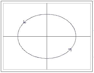
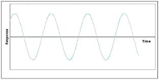
When the real part is zero, the system behaves as an undamped oscillator. This can be visualized in two dimensions as a vector tracing a circle around a point. The plot of response with time would look sinusoidal. The figures below should help in understanding.

Undamped oscillation is common in many control schemes arising out of competing controllers and other factors. Even so, this is usually undesirable and is considered an unstable process since the system will not go back to steady state following a disturbance.

Negative Real Part

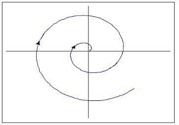
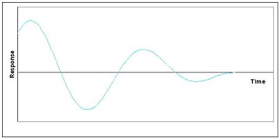
When the real part is negative, then the system is stable and behaves as a damped oscillator. This can be visualized as a vector tracing a spiral toward the fixed point. The plot of response with time of this situation would look sinusoidal with ever-decreasing amplitude, as shown below.

This situation is what is generally desired when attempting to control a process or unit. This system is stable since steady state will be reached even after a disturbance to the system. The oscillation will quickly bring the system back to the setpoint, but will over shoot, so if overshooting is a large concern, increased damping would be needed.

While discussing complex eigenvalues with negative real parts, it is important to point out that having all negative real parts of eigenvalues is a necessary and sufficient condition of a stable system.

Complex Part of Eigenvalues

As previously noted, the stability of oscillating systems (i.e. systems with complex eigenvalues) can be determined entirely by examination of the real part. Although the sign of the complex part of the eigenvalue may cause a phase shift of the oscillation, the stability is unaffected.

Real Eigenvalues

We've seen how to analyze eigenvalues that are complex in form, now we will look at eigenvalues with only real parts.

Zero Eigenvalues

If an eigenvalue has no imaginary part and is equal to zero, the system will be unstable, since, as mentioned earlier, a system will not be stable if its eigenvalues have any non-negative real parts. This is just a trivial case of the complex eigenvalue that has a zero part.

Positive Eigenvalues

When all eigenvalues are real, positive, and distinct, the system is unstable. On a gradient field, a spot on the field with multiple vectors circularly surrounding and pointing out of the same spot (a node) signifies all positive eigenvalues. This is called a source node.

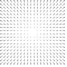
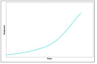
Graphically, real and positive eigenvalues will show a typical exponential plot when graphed against time.

Negative Eigenvalues

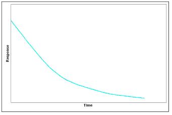
When all eigenvalues are real, negative, and distinct, the system is unstable. Graphically on a gradient field, there will be a node with vectors pointing toward the fixed point. This is called a sink node.

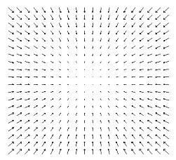
Graphically, real and negative eigenvalues will output an inverse exponential plot.

Positive and Negative Eigenvalues

If the set of eigenvalues for the system has both positive and negative eigenvalues, the fixed point is an unstable saddle point. A saddle point is a point where a series of minimum and maximum points converge at one area in a gradient field, without hitting the point. It is called a saddle point because in 3 dimensional surface plot the function looks like a saddle.

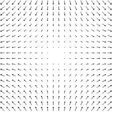
Repeated Eigenvalues

If the set of eigenvalues for the system has repeated real eigenvalues, then the stability of the critical point depends on whether the eigenvectors associated with the eigenvalues are linearly independent, or orthogonal. This is the case of degeneracy, where more than one eigenvector is associated with an eigenvalue. In general, the determination of the system's behavior requires further analysis. For the case of a fixed point having only two eigenvalues, however, we can provide the following two possible cases. If the two repeated eigenvalues are positive, then the fixed point is an unstable source. If the two repeated eigenvalues are negative, then the fixed point is a stable sink.

Summary of Eigenvalue Graphs

Below is a table summarizing the visual representations of stability that the eigenvalues represent.

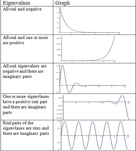
Note that the graphs from Peter Woolf's lecture from Fall'08 titled Dynamic Systems Analysis II: Evaluation Stability, Eigenvalues were used in this table.

Another method of determining stability

The process of finding eigenvalues for a system of linear equations can become rather tedious at times and to remedy this, a British mathematician named Edward Routh came up with a handy little short-cut.

First, recall that an unstable eigenvalue will have a positive or zero real part and that a stable eigenvalue will have a negative real part.

The first test is to take an n-th degree polynomial of interest:

\[P(\lambda)=a_{0} \lambda^{n}+a_{1} \lambda^{n-1}+\cdots+a_{n-1} \lambda+a_{n} \nonumber \]

and look to see if any of the coefficients are negative or zero. If so, there is at least one value with a positive or zero real part which refers to an unstable node.

The way to test exactly how many roots will have positive or zero real parts is by performing the complete Routh array. Referring to the previous polynomial, it works as follows:

Row
1
2
3
4
n-1
n
n+1

An array of n+1 rows and the coefficients placed as above. After the first two rows, the values are obtained as below:

\[b_{1}=\frac{a_{1} a_{2}-a_{0} a_{3}}{a_{1}}, b_{2}=\frac{a_{1} a_{4}-a_{0} a_{5}}{a_{1}}, b_{3}=\frac{a_{1} a_{6}-a_{0} a_{7}}{a_{1}}, \cdots c_{1}=\frac{b_{1} a_{3}-a_{1} b_{2}}{b_{1}}, c_{2}=\frac{b_{1} a_{5}-a_{1} b_{3}}{b_{1}}, c_{3}=\frac{b_{1} a_{7}-a_{1} b_{4}}{b_{1}}, \cdots \nonumber \]

Routh’s theorem says:

Routh’s Theorem

1. For all of the roots of the polynomial to be stable, all the values in the first column of the Routh array must be positive.
2. If any of the values in the first column are negative, then the number of roots with a positive real part equals the number of sign changes in the first column.

So considering the following example,

\[f(x)=9 x^{4}+14 x^{3}+7 x+10 \nonumber \]

Preliminary test: All of the coefficients are positive, however, there is a zero coefficient for x² so there should be at least one point with a negative or zero real part.

Routh array:

Row
1	\[\\;9 \qquad \quad 0 \qquad \quad 10 \nonumber \]
2	\[\\; 14 \qquad \; \; 7 \nonumber \]
3
4
5

Since Row 3 has a negative value, there is a sign change from Row 2 to Row 3 and again from Row 3 to Row 4. Thus, there are 2 roots with positive or zero real part.

Stability Summary

The following image can work as a quick reference to remind yourself of what vector field will result depending on the eigenvalue calculated.

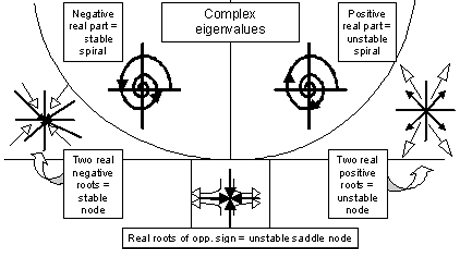
The table below gives a complete overview of the stability corresponding to each type of eigenvalue.

Eigenvalue Type	Stability	Oscillatory Behavior	Notation
All Real and +	Unstable	None	Unstable Node
All Real and -	Stable	None	Stable Node
Mixed + & - Real	Unstable	None	Unstable saddle point
+a + bi	Unstable	Undamped	Unstable spiral
-a + bi	Stable	Damped	Stable spriral
0 + bi	Unstable	Undamped	Circle
Repeated values	Depends on orthogonality of eigenvectors

Advantages and Disadvantages of Eigenvalue Stability

There are several advantages of using eigenvalues to establish the stability of a process compared to trying to simulate the system and observe the results. However, there are situations where eigenvalue stability can break down for some models.

Advantages

1. High accuracy for linear systems.
2. General method that can be applied to a variety of processes.
3. Can be used even if all variables are not defined, such as control parameters.

Disadvantages

1. Only applicable for linear models.
2. Linear approximations of nonlinear models break down away from the fixed point of approximation.

Example \(\PageIndex{1}\)

For the system described by:

\[\begin{align*} \frac{d x}{d t} &=y \\[4pt] \frac{d y}{d t} &=2 x+y \end{align*} \nonumber \]

Find the fixed points and determine their stability.

Solution

Step 1. Determining the fixed points

At the fixed points, nothing is changing with respect to time. Therefore, set the derivatives to zero to find the fixed points.

\[\begin{array}{c}
0=y \\
0=2 x+y
\end{array} \nonumber \]

Solving these two equations simultaneously, we see that we have one fixed point at {0,0}

Step 2. Determine the eigenvalue of this fixed point

First, let us rewrite the system of differentials in matrix form.

\[\left[\begin{array}{l}
\frac{d x}{d t} \\
\frac{d y}{d t}
\end{array}\right]=\left[\begin{array}{ll}
0 & 1 \\
2 & 1
\end{array}\right]\left[\begin{array}{l}
x \\
y
\end{array}\right] \nonumber \]

Next, find the eigenvalues by setting \(\operatorname{det}(A-\lambda I)=0\)

Using the quadratic formula, we find that and

Step 3. Determine the stability based on the sign of the eigenvalue

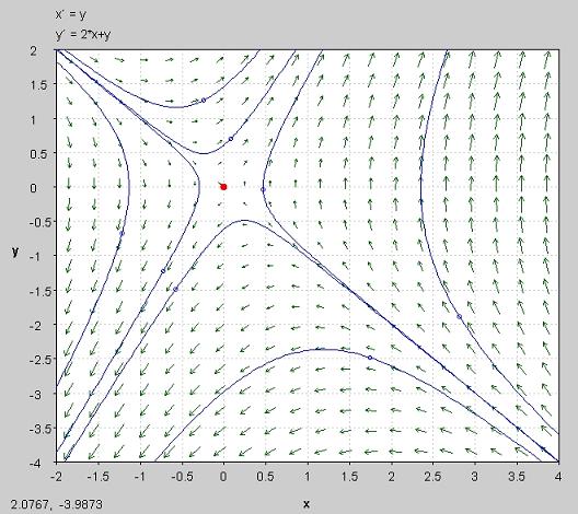
The eigenvalues we found were both real numbers. One has a positive value, and one has a negative value. Therefore, the point {0, 0} is an unstable saddle node.

The stability can be observed in the image below. The fixed point is seen at (0,0). All solutions that do not start at (0,0) will travel away from this unstable saddle point. The solution was found by using the two-dimensional system in PPlane 2005.10 PPlane.

Example \(\PageIndex{2}\)

Determine the Routh array and the number of positive or zero roots of the following equation.

\[f(x)=6 x^{5}+12 x^{4}+5 x^{3}+3 x^{2}+17 x \nonumber \]

Solution

Routh Array:

Row
1	\[\\;6 \qquad \quad 5 \qquad \quad 17 \nonumber \]
2	\[\\;12 \quad \qquad 3 \qquad \quad 0 \nonumber \]
3
4
5
6

Since you go from a positive value in row three, to a negative value in row four, and back to a positive value in row five, you will have a positive or zero real part for two of your roots.

Example \(\PageIndex{1}\)

Use Mathematica to find the eigenvalues of the system defined by:

\[\begin{align*}
\frac{d x_{1}}{d t} &=8 x_{1}+15 x_{2}-3 x_{3}+7 x_{4}+2 x_{5} \\[4pt]
\frac{d x_{2}}{d t} &=-22 x_{1}-21 x_{2}+3 x_{3}-12 x_{4}+11 x_{5} \\[4pt]
\frac{d x_{3}}{d t} &=10 x_{1}+6 x_{2}+24 x_{3}+3 x_{4}-6 x_{5} \\[4pt]
\frac{d x_{4}}{d t} &=0 x_{1}-2 x_{2}+21 x_{3}+0 x_{4}+4 x_{5} \\[4pt]
\frac{d x_{5}}{d t} &=4 x_{1}+9 x_{2}+x_{3}-22 x_{4}-7 x_{5}
\end{align*} \nonumber \]

And comment on the stability of this system

Solution

The matrix that corresponds with this system is the square matrix:

\[\left[\begin{array}{ccccc}
8 & 15 & -3 & 7 & 2 \\
-22 & -21 & 3 & -12 & 11 \\
10 & 6 & 24 & 3 & -6 \\
0 & -2 & 21 & 0 & 4 \\
4 & 9 & 1 & -22 & -7
\end{array}\right] \nonumber \]

Using the Eigenvalues[ ] function in Mathematica the input is:

In[1]:= Eigenvalues[

ParseError: EOF expected (click for details)

Callstack:
    at (Bookshelves/Industrial_and_Systems_Engineering/Chemical_Process_Dynamics_and_Controls_(Woolf)/10:_Dynamical_Systems_Analysis/10.04:_Using_eigenvalues_and_eigenvectors_to_find_stability_and_solve_ODEs), /content/body/div[6]/div[2]/section[3]/div/div/p[4]/span/span, line 1, column 2

]

In[2]:= N[%] This step produces numerical results

The output contains the 5 eigenvalues:

out[2]:= {27.0612, -10.7653 + 10.0084, -10.7653 - 10.0084, -0.765272 + 7.71127, -0.765272 - 7.71127}

So the five eigenvalues are:

27.0612

-10.7653 + 10.0084

-10.7653 - 10.0084

-0.765272 + 7.71127

-0.765272 - 7.71127

Looking at these eigenvalues it is clear that the system as a whole is unstable. This is because one of the eigenvalues has a positive real part.

Multiple Choice Question 1

A system is stable if and only if all of the system's eigenvalues:

1. a. are real
2. b. are complex
3. c. have negative real parts
4. d. have negative imaginary parts

Answer: c

Multiple Choice Question 2

What would the following set of eigenvalues predict for the system's behavior?

\[-4,-2+3 i,-2-3 i, 3 \nonumber \]

a. An unstable oscillation

b. A damped oscillation

c. An undamped oscillation

d. A source

e. A saddle point

Answer: d

References

• Kravaris, Costas. Chemical Process Control: A Time Domain Approach.
• Liptak, Bela G., Process Control and Optimization. Vol. II. New York: Taylor & Francis.

Contributors

• Daniel Katzman, Jessica Moreno, Jason Noelanders, and Mark Winston-Galant