10.6: Root Locus Plots - Effect of Tuning
- Page ID
- 22505
Introduction
Root locus plots show the roots of the systems characteristic equation, (i.e. the Laplacian), as a function of the control variables such as \(Kc\). By examining these graphs it is possible to determine the stability of different values of the control variable. A typical transfer function is of the form \(G(s) = Y(s)/U(s)\).
- Poles: U(s) = 0
- Zeros: Y(s) = 0
In other words, after factorization the poles are the roots of the denominators and the zeros are the roots of the numerator. Stability only depends on the value of the poles. The system is stable for all values of the control variables that result in the value of the real part of every pole value being less than zero.The lines of a Root locus plot display the poles for values of the control variable(s) from zero to infinity on complex coordinate system. These plots will always have a line of symmetry at \(i = 0\).
Closed-loop vs. Open-loop
A closed-loop system uses feedback control where the output has an effect on the input. With a closed-loop, oscillations are usually introduced, and therefore can become unstable. Unlike the open-loop systems, the closed-loop incorporates valves and controllers.
In an open-loop system, the output is not compared with and has no effect on the input. In an open-loop system, oscillations are not introduced and therefore cannot become unstable. An open-loop system, however, can be inaccurate because it does not take into account the control dynamics. Open-loop systems will include feed forward control schemes or timed control schemes. The two diagrams below depict this difference when trying to control the temperature in your apartment. (Click on images for increased resolution).
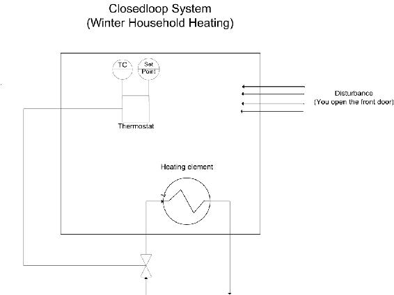
In this diagram a thermostat presents feedback to the heater to turn it on or off.
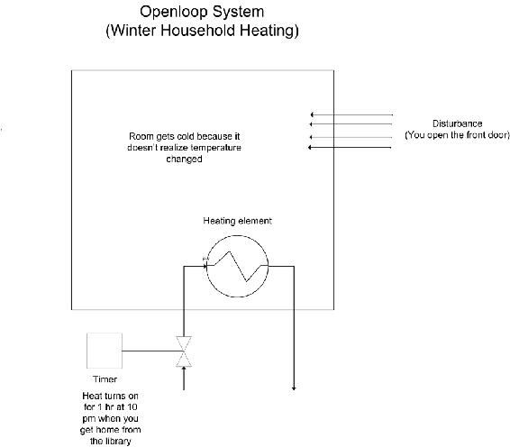
Since the heater only turns on at 10 pm, it assumes that the amount of time you open the door will be the same each day. It is considered an open system since the temperature in the room is independent of the heater controller.
Note that all the examples presented in this web page discuss closed-loop systems because they include all systems with feedback.
Complex Coordinate Systems
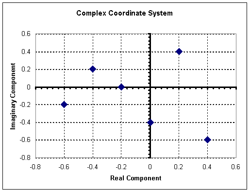
Root locus plots are a plot of the roots of a characteristic equation on a complex coordinate system. A complex coordinate system allows the plotting of a complex number with both real and imaginary parts. The real component is plotted on the x-axis and the imaginary component is plotted on the y-axis. When creating root locus plots imaginary roots must be solved for. These imaginary roots come in complex conjugate pairs (this can be seen below in the section on "Plotting Poles on a Complex Coordinate System to make Root Locus Plot").
For example a plot of the following complex numbers is shown below. These complex numbers can be broken into the real and imaginary components to make it easier to plot.

Developing a Characteristic Equation
Although the focus of this article is to discuss root locus plots, it is necessary to mention briefly how to determine the characteristic equation for a system in order to obtain the root locus plot. In general, most chemical engineering processes can be described by a system of ordinary differential equations. Follow the following steps to determine the characteristic equation for the system (which will allow you to develop a root locus plot).
- If the ODEs are not linear, linearize them. (See this link for more information on linearizing ODEs <controls.engin.umich.edu/wiki/index.php/LinearizingODEs>)
- After linearizing the ODEs, use matrix algebra to find the eigenvalues of your system. Be careful here not to insert numerical values for your control parameters, (e.g. leave Kc as Kc, not Kc=1). (For more information on finding eigenvalues <controls.engin.umich.edu/wiki/index.php/EigenvaluesEigenvectors>)
- The polynomial equation obtained for the eigenvalue should contain lambda and the control parameters. This equation is the characteristic equation. Obtain solutions to this equation by setting values for the control parameters and solving for the eigenvalues. The roots obtained will be used to create the root locus diagram.
This 3-step process is valid to obtain a characteristic equation for any closed loop control system. A more traditional method to develop characteristic equations is by applying Laplace transforms.
Laplace Transforms
Laplace transforms are a method to change linear ordinary differential equations into transfer function. All transfer functions used in root locus plots are independent of time because the \(L[f(t)] ≣ F(s)\). Formally, the equation below shows that the time function is integrated, leaving only the variable \(s\).
\[\mathbf{F}(\mathbf{s})=\int_{0}^{\infty} f(t) e^{-s t} d t \nonumber \]
s is a complex number, therefore allowing us to construct complex coordinate system graphs. The exact solution to most disturbances and controllers can be found in any controls book. Please always refer to your Ordinary differential equations mathematics book for more information on Laplace transforms.
The stability of the series chemical reactors is to be determined. The reactors are well mixed and isothermal, and the reaction is first-order in component A. The outlet concentration of the second reactor is controlled with a PI feedback algorithm that manipulates the flow of the reactant, which is very much smaller than the flow of the solvent. The sensor and final element are assumed fast, and process data is as follows.
Process
- V= 5m3
- Fs=5m3/min >> FA
- k = 1 min-1
- vs= 50% open
- CA0 = 20 mole/m3
- CA0(s)/v(s) = Kv= 0.40 (mole/ m3) (%open)
- PI Controller Kc = ?? Tf = 1 min
Formulation The transfer function for the process and controller are
\[G_{y}(s)=\frac{K_{y}}{(\tau s+1)(\tau s+1)} \nonumber \]
\[G_{c}(s)=K_{c}\left(1+\frac{1}{T_{f} s}\right) \nonumber \]
\[K_{y}=K_{v}\left(\frac{F}{F+V k}\right)=0.1 \frac{m o l e / m^{3}}{\%} \nonumber \]
\[\tau=\frac{V}{F+V R}=0.5 \mathrm{min} \nonumber \]
The individual transfer functions can be combined to give the closed-loop transfer function for a set point change, which includes the characteristic equation. (where CV= Control variable & SP = set-point signal)
\[\frac{C V(s)}{S P(s)}=\frac{G_{p}(s) G_{v}(s) G_{c}(s)}{1+G_{r}(s) G_{v}(s) G_{c}(s) G_{s}(s)}=\frac{K_{p}\left(1+\frac{1}{s}\right) \frac{0.1}{(0.5 s+1)^{2}}}{1+K_{p}\left(1+\frac{1}{s}\right) \frac{0.1}{(0.5 s+1)^{2}}} \nonumber \]
Characteristic equation
\[0=1+K_{p}\left(1+\frac{1}{s}\right) \frac{0.1}{(0.5 s+1)^{2}} \nonumber \]
Root Locus Diagrams
Root Locus plots are a method of evaluating the behavior of a control system. The creation of a root locus plot begins by determining the poles of the control system for a given set of control parameters. These poles are then plotted on a complex coordinate system as seen in the previous section and analyzed to determine the behavior of the system.
Determining the Poles of a Control System
The “poles” of a system are the roots of the demoninator of the transfer function. In other words the poles are the values of "s" when the transfer function go to infinity (when the demoninator equals zero). For a system of differential equations, poles are the eigenvalues of the equation system. Consider the following solution to a system of differential equations:
\[f(s) = 48s^3 + 44s^2 + 12s + 1 \label{eq1} \]
This equation is a third order polynomial, therefore it will have three poles (be aware that some of these poles may be imaginary numbers). These poles can be obtained by factoring the expression or using a computer program such as Maple. The three poles, or roots, of this equation are s = -0.167, -0.25, -0.5.
For a system of differential equations, finding the eigenvalues can be time consuming and the use of Matlab, Maple, or Mathematica is more efficient. One method would be to use the Mathematica eigenvalues[] function to solve the system for you. This function is explained in Eigenvalues and Eigenvectors section of the wiki text.
Plotting Poles on a Complex Coordinate System to make Root Locus Plot
A root locus plot is created by plotting the resulting poles on a complex coordinate system. For system of P-only control, the governing differential equations will depend on the proportional gain, Kc. Consider the following solution to a system of differential equations:
\[f(s)=48 s^{3}+44 s^{2}+12 s+1+6 Kc \label{2} \]
Notice that Kc is a term in this equation. Therefore, there exists a set of poles for each value of Kc. If Kc = 0, then equation #2 reduces to equation #1, and poles are as listed above. Table 1 lists the three poles of the system for given values of Kc. These poles were calculated using a computer algebra system because it is impractical to try and evaluate these functions with analytical methods.
Table 1- Poles of Characteristic Equation
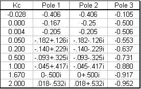
To create a root locus plot, each pole is broken down into its real (x-axis) and imaginary (y-axis) component (Table 2):
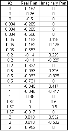
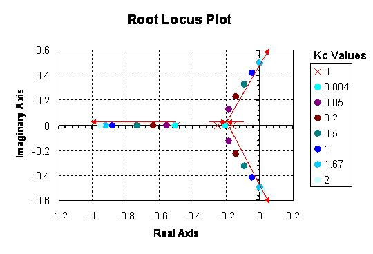
By convention, red arrows are drawn on the plot in the direction of increasing Kc values. They help to illustrate how the roots of the system vary by changing the Kc value. Also by convention, the points in which Kc = 0 are represented with ‘x’ marks instead of dots.
Interpreting a Root Locus Diagram
The primary use of a Root Locus Diagram is to evaluate how differing values of Kc affect the stability and behavior of a control system.
The stability of the control system depends on the sign of the real component of the pole. If the real components of all poles are negative, then the system is said to be stable for that value of Kc. If the real component of the pole is positive, the system is unstable for that value of Kc, meaning the output signal will diverge from the set point.
The behavior of the control system depends on the presence of an imaginary component of the pole. If any of the three poles contains an imaginary number component, then that value of Kc will cause the output signal to oscillate. If all of the poles are real (contain no imaginary components), the output signal will not oscillate at that Kc value.
Please refer back to the Root Locus diagram in Figure 1. The system becomes unstable (i.e. the real component of the poles becomes positive) for Kc > 1.67 and Kc < 0. Within the range of stability, no oscillations (i.e. no imaginary component) are observed when 0 < Kc < 0.004.
Root Locus Diagrams for PID Control
Root Locus diagrams are much more difficult to create for PID control. The characteristic equation will contain unknown variables Kc, Ti, and Td. Therefore, each point on the Root Locus Diagram will represent a set of tuning parameters. In order to show the progression as each tuning parameter changes, the resulting diagram will be a three-dimensional surface plot. Due to the complexity of this diagram, we will not create one, as it is beyond the scope of this text. However, stability analysis can still be applied to the characteristic equation. Take for example Equation \ref{eq3}:
\[f(s)=\frac{48 s^{3}+44 s^{2}+12 s+1+6 K c}{T i+3 T d} \label{eq3} \]
In this theoretical instance, equation 3 is the characteristic equation governing the same system mentioned above, only now with PID control. Notice the additional presence of the Ti and Td terms. Under P- only control, this system was stable for Kc values between 0 and 1.67. Will the same be true if this system were tuned with PID control?
Let’s suppose we want to test the conditions Kc = 1.0, Ti = 0.3 and Td = 0.1. These values were randomly chosen. Using a computer software package, the three roots were determined to be: r1 = -0.827, r2 = -0.044 + 0.417i, r3 = -0.044 – 0.417i. Therefore, since the real components are all negative, the system is still stable. Since complex roots are present, the response is expected to oscillate around the set point.
Creating Root Locus Plots with Mathematica
Mathematica allows you to develop root locus plots for polynomials since the math involved in solving for the solutions can become very tedious. Before you are able to obtain the root locus plot, you need to solve for the roots. We will use the same equation as was used in the “Determining the Poles of a Control System” section.
\[f(s) = 48s^3 + 44s^2 + 12s + 1 + 6K_c \nonumber \]
The Solve[ ] function can be used to determine the roots, both real and imaginary, for each corresponding Kc value. The syntax in Mathematica is shown below for the specified equation when Kc = 0. It is important to note that in order to obtain an output you must press “Shift Enter.”

The following is just to show how Mathematica formats the output when \(Kc ≠ 0\) and when there are imaginary roots. In this case, \(Kc = -0.167\).

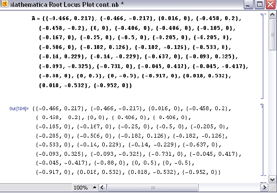
This can be done for all Kc values to obtain the corresponding real and imaginary roots. After all of the roots have been calculated, a table can be made to format the real roots (x axis) verses imaginary roots (y axis). When the syntax, A={{x,y}{a,b}…}, is used, you are inputting all of the x and y values and naming those values A. When you call A in the TableForm[ ] function, the table will be made according to all of the x and y values input into A. The syntax and corresponding outputs are shown below.
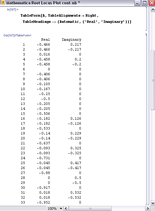
In order to produce the table shown above, you only need TableForm[A] and nothing else. The other descriptions (ie. TableAlignments and TableHeadings) are just used for formatting purposes.
Once the real (x) and imaginary (y) roots have been determined and put into table format for your equation, the ListPlot[ ] function can be used to develop your root locus diagram by calling A.
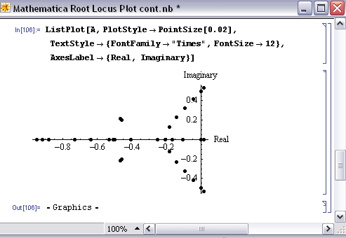
As you can see, the ListPlot[ ] function returned the same plot as shown in the “Complex Coordinate System to make Root Locus Plot” section (this plot was created in Excel). The arrows are not shown in this Mathematica plot; however the Excel plot shows the direction of increasing Kc values to show how the roots of the system vary by changing the Kc values.
The Mathematica Help Browser is a very useful tool for understanding the syntax. For example, when using the ListPlot[ ] function you can search how to label the axes and how to make the points larger (more visible) on the plot. The following examples are used to illustrate the use of root locus plots. Click the following link if you would like to access the actual Mathematica file: Media:RLPFinalaa.nb
Second Plot Method Using Arrays
The goal here is to be able to understand exactly what is happening with these Mathematica inputs in order to get a better grasp on the outputs. Basically, once you have found the Eigenvalues of the system, which examples can be found for in other areas of the wiki, we then want to solve explicitly for them. After we solve for the Eigenvalue in terms of the variables, we can create an array by varying this value and solving for the real and imaginary terms of the Eigenvalues.
Eigenvalue Outputs in Mathematica
The Eigenvalues can either be returned as a function of 'l', which is the designation of the Eigenvalue or simply as a complex function in terms of variables. When returned as a function of 'l' there will be a polynomial input that has to be simplified to find 'l' as a function of the variable. In this case: Kc.

This example is taken directly from lecture 17 and its supplementary Mathematica file. What is happening here is that the Jacobian was inputted, and there were multiple eigenvalue arrays that were found. The last array has three complex polynomial functions that equal to 0. The last line is simplifying them, solving for 'l'. This is putting the simplified Eigenvalues into the array 'ss'.
Another output of Eigenvalues is simply in the form of complex numbers themselves. Rather than worry about the simplification steps, these Eigenvalues can be directly inputted as a complex number into an array, again termed 'ss':

This is a variation of the sample in lecture 17.
Plot Array Creation
Now that we have seen the two ways of Eigenvalue array creation, we can use these to create another array that will be the points for the plot. Here we will be substituting in values of the variable Kc to find different values of the Eigenvalues, which will give us information on stability changes as Kc changes.
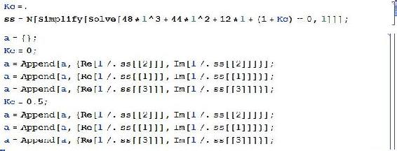
In the example above, 'ss' is in the form :
Callstack:
    at (Bookshelves/Industrial_and_Systems_Engineering/Chemical_Process_Dynamics_and_Controls_(Woolf)/10:_Dynamical_Systems_Analysis/10.06:_Root_locus_plots-_effect_of_tuning), /content/body/div[6]/div[2]/p[3]/span, line 1, column 10
However, not all Eigenvalue arrays will have the same number of Eigenvalues. For example, as mentioned in the above paragraph, 'ss' is in the form :
Callstack:
    at (Bookshelves/Industrial_and_Systems_Engineering/Chemical_Process_Dynamics_and_Controls_(Woolf)/10:_Dynamical_Systems_Analysis/10.06:_Root_locus_plots-_effect_of_tuning), /content/body/div[6]/div[2]/p[4]/span, line 1, column 10

These different methods both output arrays of numbers that act essentially as 'x' and 'y' values, or in this case Real and Imaginary, for the plot. The array 'a' is plotted as such:
ListPlot[a, PlotStyle -> PointSize[0.02]]
This is inputted directly to Mathematica, which creates the Root Locus Plot.
Differential Equation Example of Root Locus Plots in Mathematica
An example problem pulled from the Fall 2008 second exam:
"You have just been put in charge of designing a large-scale bioreactor for the production of a blockbuster protein based drug. After some research, you have come up with the following model to describe the reactor system:"
\[\dfrac{dX}{dt} = − 2X + \dfrac{10 X S}{S + 2} \nonumber \]
\[\dfrac{dS}{dt} = 4 Fin − S − \dfrac{3 X S}{S + 2} \nonumber \]
\[\dfrac{dP}{dt} = 9 X − 2 P \nonumber \]
where \(X\) is the cell concentration, \(S\) is the nutrient concentration, and \(P\) is the protein product. \(Fin\) is the flow rate of nutrient into the system.
In this system there are two fixed points found by setting all the differential equations equal to zero and solving in Mathematica.


The two fixed points depend on the value of Fin and with that varying values of Fin will change eventual eigenvalues. Since this problem will eventually want root locus plots for both fixed points it is easier to save both points as parameters to be applied to general equations later. Overall it will help save the need for redundant code. The entire mathematica file being referenced in this example is available here: Media:Exam2Prob1.nb
From this point a Jacobian matrix should be created to linearize the system around the fixed points (as applied to the Jacobian). Once created the stored fixed point values for X, S, and P can be applied. Once applied, the eigenvalues for each fixed point can be solved for. These will still contain a variable 'Fin' since Fin has not been defined yet.
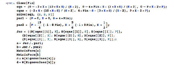
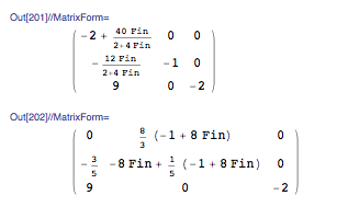
From here the Table[] function can be used to tabulate eigenvalues for various Fin values for visual sake of inspection. This is not necessary since the eigenvalue results have already been solved for in terms of Fin. To create the root locus plots, values of Fin need to be defined and applied to the eigenvalue equations with the results stored. That step is next. In this table step it is for the user's sake to see with increasing Fin values what the eigenvalues look like. The tabulated eigenvalues are stored as a matrix and displayed as such with the function 'MatrixForm[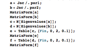
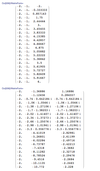
These tables make it easy to see with increasing Fin (goes from 0 to 2 down the table) what the changes are in the stability of each fixed point. The first table is the first fixed point, the second table the second FP.
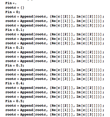
Now, to make the root locus plots, a really long string of values needs to be created in order for the real and imaginary roots to be plotted. This is a long string of code that is basically brute force. The overall action occurring here is setting Fin to a value, evaluating that Fin through the eigenvalues, and saving the real portion separate from the imaginary portion by different columns. This is repeated for as many Fin values as you desire. It is extremely repetitive, but works. After evaluating as many Fin values as you desired you can display the two columns through the ListPlot[] function. Example snippets of the code look like such:
And the ListPlot[] function can look like this:

And would make graphs like these (Fixed Point 1 on top and FP2 on bottom in this example):
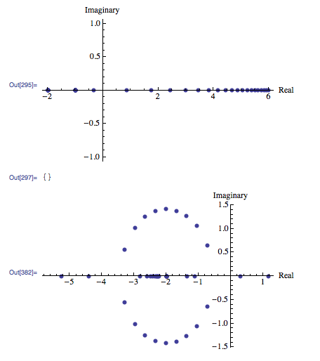
Looking back at the tables of eigenvalues the plots can be interpreted. For FP1 the values start real negative and increase to real positive. There are no imaginary values. For FP2, increasing Fin values go from real positive to negative with imaginary values occurring in the transition from low to high Fin values.
Alternative Mathematica Method
Some Mathematica 6 programs have an add-on or supplementary application known as ANALOG INSYDES which contains special options to create Root Locus Plots with ease. The Function is called RootLocusPlot. Enter the function that is to be analyzed, into Mathematica with the following format:
RootLocusPlot[tfunc,{k,k_0 ,k_1}]
tfunc is the transfer function in the frequency variable s and one real parameter k. k_0 and k_1 are the range for the real parameter k that is to be varied int he Root Locus Plot. Follow an example below.
Example: Equation to make a Root Locus Plot with:
\[H(s) = \drac{a + 2 s + s2}{10 + 3 a s + 4 s^2 + s^3} \nonumber \]
To make a Root Locus Plot follow the example code below:
H4[s_, a_] := (a + 2*s + s^2)/(10 + 3*a*s + 4*s^2 + s^3)
RootLocusPlot[H4[s, a], {a, 3, 5}]
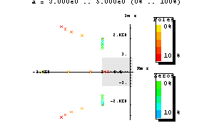 Image: Wolfram.com
Other Mathematica forms for using RootLocusPlot[]:
RootLocusPlot[func] This form displays the a pole/zero diagram of a function i.e. func without parameters k and k_1.
RootLocusPlot[rootloc] This form displays a root locus calculated with function RootLocusByQZ[].
Refer to Mathematica link for further discuss about RootLocusByQZ
Many options for the plot can be varied including the number of points, plot style, and plot color. All of these options and more can be viewed online with a Mathematica Tutorial
Creating Root Locus Plots with Matlab
Root Locus Generation in Matlab
Three matlab files have been given to obtain the root locus plot and poles of the root locus plot at specified Kc values for a specific transfer function with relative ease. These three files are polesfunction.m, transferfunction.m, and Locusplotpoles.m .[1]. The transferfunction file is where the specific transfer function should be input. As written the only line needing variation is line 4 (Gs). The polesfunction file finds the poles of the given transfer function using built in matlab utilities and needs no variation, even after changing the transfer function. The Locusplotpoles file is what is called in matlab to generate the root locus plot as well as the value of the poles and integrates the two previous files. To use this file you type in the values of the specific Kc you require the pole values for as well as a single value of Kc for which you would like to see the root locus plot. An example of the inputs to and outputs of this file are given below.
>> Locusplotpoles([0 50 100 200],0)
ans =
1.0e+002 *
Columns 1 through 3
0 -0.0020 -0.0020 + 0.0000i 0.5000 -0.0045 -0.0008 + 0.0022i 1.0000 -0.0051 -0.0004 + 0.0027i 2.0000 -0.0060 -0.0000 + 0.0034i
Columns 4 through 6
-0.0020 - 0.0000i 0 0 -0.0008 - 0.0022i -0.0020 -0.0020 + 0.0000i -0.0004 - 0.0027i -0.0020 + 0.0000i -0.0020 - 0.0000i -0.0000 - 0.0034i -0.0020 -0.0020 + 0.0000i
Column 7
0 -0.0020 - 0.0000i -0.0020 -0.0020 - 0.0000i
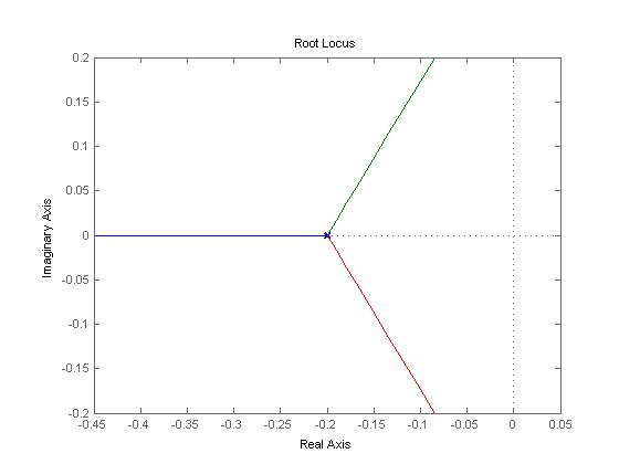
The values inside the brackets are the specific Kc values for which poles are desired. The last value is the Kc which the root locus plot will be plotted for. Notice that the value of Kc for the root locus plot to be generated in this example is zero. This is so that the entire range of Kc can be examined using the interactive graph produced by matlab. If other specific Kc plots would like to be observed this value can be changed to generate these as well. The column lines give the values of Kc input and then value of the poles for each Kc. Note that the actual values are the values matlab gives multiplied by 100.
Now that a basic understanding of root locus plots has been obtained here are a few websites which go further in depth into the underlying principles and generation of these plots. www.facstaff.bucknell.edu/mastascu/eControlHTML/RootLocus/RLocus1A.html
This site gives animated examples which progress the value of the control variable through a root locus plot to better explain the fundamental function of these plots. It would be beneficial to go through a few of these examples to observe patterns of fluctuation of the control variable. The parameters for each animation are given to the left of the frame. www.engin.umich.edu/group/ctm/rlocus/rlocus.html
This page gives examples of how you generate a root locus plot of a given transfer function using matlab. While you go through the content on this page take special notice of the fact that none of the given transfer functions have an integrated Kc variable for which to generate a locus plot. To see how these plots can are generated when a value of Kc is specified see the code of Locusplotpoles.m. For clarification on the application of root locus plots see the given examples.
Creating Root Locus plots with Excel and PPLANE
Though this tactic may remain slightly more time consuming and work involved, there is a method in computing the Root Locus plot using PPLANE and Excel. This particular model really aids in better understanding of how to read and acknowledge a Root Locus Plot, and is also useful if alternative options for making a Root Locus Plot are not currently available.
This method involves using PPLANE in order to find the eigenvalues for each equilibrium value, and then plotting these points with Excel software. In order to do this, suppose that you have the following differential equations that represent a reactor:
\[\dfrac{dX}{dt} = -X + \dfrac{2+X+Y}{Y+3} \nonumber \]
\[\dfrac{dY}{dt} = Y \times Fin+7-(2X) \nonumber \]
Graphing the following differential equations provides something similar to the following chart (a few lines were drawn, just to better show the graphs flow):
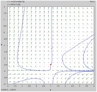
Using the ability to “Find an Equilibrium Point” in PPLANE (if you need help with PPLANE, click PhasePlaneAnalysis), one can select a particular equilibrium point on the field, and be able to provide the following results:
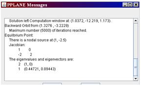
This window “pops up” in the higher left corner of the screen, when the equilibrium point is found. This window provides the eigenvalues for this equilibrium point.
Depending what you are varying (in this case, Fin), all you would have to do is enter various values of this Fin into PPLANE, and plot the new set of differential formulas. After this is done, just find the same equilibrium point, and record the new given eigenvalues in excel. These values should be entered with an x-component (in one column) and a y-component (in another column) into excel, with the following rules:
- Assuming the example 3+3i, 3-3i were given as eigenvalues.
- For any given eigenvalue, the x-value of a particular eigenvalue is the real part of that number (ie: the “3” part).
- For any given point, the y-value of a particular eigenvalue is the imaginary part of that number (ie: the “3i” part). If there is an imaginary component, ignore the “i,” though the number should be recorded in the y-component. If there is no imaginary number, the y component is zero.
- For both cases, a positive is a positive, and a negative is a negative. Remember: imaginary numbers have 2 parts, a positive and negative “i” value.
These points are simply recorded according to these rules, then the points are plotted against each other, with x components on the x-axis, and the y in the y-axis. Here is an example of an excel diagram, taken from the proposed diagram:
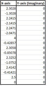
And, the excel data is then plotted, x against y, and is shown below:
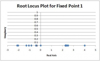
As you can see, this particular model did not have any imaginary data. The root locus plot has been formed, and for all accounts of Fin, the eigenvalues are along the x-axis for the root locus plot.
Practical Application
In the past, it was necessary for engineers to master the techniques required to efficiently construct root locus diagrams. In today's engineering world, this is not the case for one of two reasons. In many instances, root locus diagrams are not used industrially because they require models of the system which are generally not available. If a model is available to develop a root locus diagram, there are computer applications that can develop the diagrams much faster than a person. Thus, energy and effort should be placed on understanding and interpreting a root locus diagram and understanding the general rules of stability for a root of the characteristic equation.
Given the following table of roots to the characteristic equation for a system:

- Construct a root locus plot (Making the plot by hand initially may give some a better understanding of what is going on as you will see the changes in the plot as you add each set of roots).
- Determine the ranges of Kc that would lead to the following system responses: no oscillations, dampened oscillations, stable oscillations & unstable oscillations. Also, sketch what the output response would look like for a given step change in input for each range of Kc.
- How would the roots to the characteristic equation be different if this were PI control?
Solution
1) Root locus plot:
First, we break the roots into their imaginary and real components:

Then, we plot each point on a complex coordinate system (x-axis = real componebt, y-axis = imaginary component).
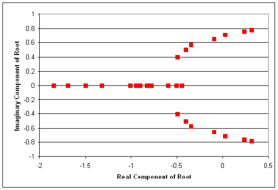
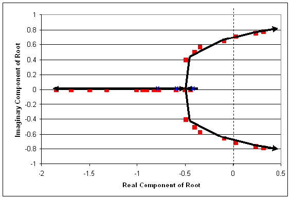
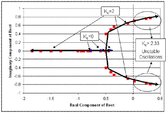
Also, it is useful to add lines tracing the path of increasing Kc. These lines are added below. Also, the points where Kc= zero are generally labeled with an x. This has also been done in the figure below.
2) Ranges of Kc with explanations:
We know that the range where there will be no oscillatory response is when Kc provides all real roots. This occurs when Kc is between 0 and 0.66. (Sketch will look like figure a in the "interpreting a root locus diagram" section above).
Also, Kc yields dampened oscillations when the two of the roots of the characteristic equation are complex with negative real components. This occurs when Kc is greater than 0.66 but less than 2.33. (Sketch will look like figure b in the "interpreting a root locus diagram" section above).
Unstable oscillations are achieved when two of the roots yield complex numbers with positive real components. This occurs when Kc is greater than 2.33. Graphically, we see that when the points move past the dashed line, we will have unstable oscillations. This is represented in the figure below. (Sketch will look like figure c in the "interpreting a root locus diagram" section above).
Based on the data provided, our best assumption is that at a Kc just below 2.33, we will be able to achieve stable oscillations. When Kc = 2.33 the real component of the complex root is 0.02 (slightly greater than zero). Ideally, we will achieve stable oscillations when the real component of the complex number is zero. (Oscillations should be consistent in magnitude).
Lastly, it is a good idea to label some values of Kc on the root locus plot. This will help orient the reader when they are trying to determine which point correspond to different values of Kc.
3) If this were PI control, each root to the characteristic equation would be accompanied by not only a Kc value but also a value for integral control parameter, KI.
You've been recently hired at MichChem Controls. In your first week at the company, a virus spreads through the computer network, effectively disabling most of the computational programs. Fortunately, the virus was halted before it was able to disable Mathematica. Shortly after the chaos from the virus subsides, your boss needs to know how to use Mathematica to create a root locus plot for several new Proportional only level control systems that are being tested. Being the highly skilled engineer that you are, he doesn't want you to waste time developing the root locus plots, rather, he wants you to write out example code, with a brief description that someone else could use to develop the root locus plot.
The general characteristic equation for the new level control systems is:
\[f(s) = Ax^3 + Bx^2 - Cx + D +EK_c \nonumber \]
Please, provide your boss with an example of the exact script that would need to be entered into Mathematica in order to develop the root locus plot. You should also brief descriptions explaining what the code does and what steps would need to be repeated to develop the plot.
Solution
First, the user should develop a table of roots for the characteristic equation. This can be done using the solve function in Mathematica. The code would appear like this for Kc = 0.
(note: the In[#] appears for each new line of code. This will not be typed in by the user.)
In[1]:= Solve[Ax^3 +Bx^2-Cx+D+E*(0)==0,x]
This should be repeated for Kc = 0.1, 0.15, 0.225, 0.5, 0.75, 1.5, etc. (until the roots of the equation begin to yield two complex solutions whose real components are positive). After a sufficient number of roots have been obtained for the characteristic equation at different values of Kc, these will need to be tabulated. To develop a table of data in Mathematica input the following code:
In[2]:= A =
Callstack:
    at (Bookshelves/Industrial_and_Systems_Engineering/Chemical_Process_Dynamics_and_Controls_(Woolf)/10:_Dynamical_Systems_Analysis/10.06:_Root_locus_plots-_effect_of_tuning), /content/body/div[11]/section[2]/div/div/p[5]/span, line 1, column 6
This tabulates the real components and the imaginary components at each value of Kc. Once all of the values are tabulated, the root locus plot can be developed using the ListPlot function.
In[3]:= ListPlot[A, PlotStyle -> PointSize[0.02]
This will plot all of the tabulated data in In[2] which is the root locus plot.
A root locus plot is used to:
- Identify the solutions to the characteristic transfer function.
- Show the response time of the feedback system to a disturbance.
- Graphically illustrate the effect of Kc on the dynamic characteristics of the feedback system.
- Choose the optimal Kc for the feedback system.
- Answer
-
c
When a root is complex with positive real parts, the oscillations are:
- Decreasing
- Increasing
- Unstable
- A & C
- B & C
- Answer
-
e
References
- Luyben, Michael L.; Luyben, William L. "essential of Process Control". McGraw-Hill:New York, 1997.
- Marlin, Thomas E. "Process Control: Designing Processes and Control Systems for Dynamic Performace 2nd Edition". McCGraw-Hill: New York, 2000.
- Ogunnaike, Babatunde A.; Ray, W. Harmon. Process Dynamics, Modeling, and Control. New York Oxford: Oxford UP, 1994. 488-507.
- Riggs, James B.; Karim, M. Nazmul. Chemical and Bio-Process Control. 3rd ed. Ferret. 279-295.
- Luyben, Michael L.; Luyben, William L.; Tyreus, Bjorn D. "Plantwide Process Control". Mcgraw-Hill:New York, 1999.
- Seborg, Dale E.; Edgar, Thomas F.; Mellichamp, Duncan A. "Process Dynamics and Control". John Wiley and Sons, Inc. 2004.
- www.engin.umich.edu/group/ctm/rlocus/rlocus.html as viewed 10/23/2007
- www.facstaff.bucknell.edu/mastascu/eControlHTML/RootLocus/RLocus1A.html as viewed 10/23/2007
Contributors and Attributions
- Authors: Halley Crast, Andrew Laskowski, Maurice Telesford, Emily Yatch
- Stewards: Victoria Cardine, Anthony Campell, David Hines, Stephen Kerns


