11.2: Feed Forward Control
- Page ID
- 22508
\( \newcommand{\vecs}[1]{\overset { \scriptstyle \rightharpoonup} {\mathbf{#1}} } \)
\( \newcommand{\vecd}[1]{\overset{-\!-\!\rightharpoonup}{\vphantom{a}\smash {#1}}} \)
\( \newcommand{\dsum}{\displaystyle\sum\limits} \)
\( \newcommand{\dint}{\displaystyle\int\limits} \)
\( \newcommand{\dlim}{\displaystyle\lim\limits} \)
\( \newcommand{\id}{\mathrm{id}}\) \( \newcommand{\Span}{\mathrm{span}}\)
( \newcommand{\kernel}{\mathrm{null}\,}\) \( \newcommand{\range}{\mathrm{range}\,}\)
\( \newcommand{\RealPart}{\mathrm{Re}}\) \( \newcommand{\ImaginaryPart}{\mathrm{Im}}\)
\( \newcommand{\Argument}{\mathrm{Arg}}\) \( \newcommand{\norm}[1]{\| #1 \|}\)
\( \newcommand{\inner}[2]{\langle #1, #2 \rangle}\)
\( \newcommand{\Span}{\mathrm{span}}\)
\( \newcommand{\id}{\mathrm{id}}\)
\( \newcommand{\Span}{\mathrm{span}}\)
\( \newcommand{\kernel}{\mathrm{null}\,}\)
\( \newcommand{\range}{\mathrm{range}\,}\)
\( \newcommand{\RealPart}{\mathrm{Re}}\)
\( \newcommand{\ImaginaryPart}{\mathrm{Im}}\)
\( \newcommand{\Argument}{\mathrm{Arg}}\)
\( \newcommand{\norm}[1]{\| #1 \|}\)
\( \newcommand{\inner}[2]{\langle #1, #2 \rangle}\)
\( \newcommand{\Span}{\mathrm{span}}\) \( \newcommand{\AA}{\unicode[.8,0]{x212B}}\)
\( \newcommand{\vectorA}[1]{\vec{#1}} % arrow\)
\( \newcommand{\vectorAt}[1]{\vec{\text{#1}}} % arrow\)
\( \newcommand{\vectorB}[1]{\overset { \scriptstyle \rightharpoonup} {\mathbf{#1}} } \)
\( \newcommand{\vectorC}[1]{\textbf{#1}} \)
\( \newcommand{\vectorD}[1]{\overrightarrow{#1}} \)
\( \newcommand{\vectorDt}[1]{\overrightarrow{\text{#1}}} \)
\( \newcommand{\vectE}[1]{\overset{-\!-\!\rightharpoonup}{\vphantom{a}\smash{\mathbf {#1}}}} \)
\( \newcommand{\vecs}[1]{\overset { \scriptstyle \rightharpoonup} {\mathbf{#1}} } \)
\(\newcommand{\longvect}{\overrightarrow}\)
\( \newcommand{\vecd}[1]{\overset{-\!-\!\rightharpoonup}{\vphantom{a}\smash {#1}}} \)
\(\newcommand{\avec}{\mathbf a}\) \(\newcommand{\bvec}{\mathbf b}\) \(\newcommand{\cvec}{\mathbf c}\) \(\newcommand{\dvec}{\mathbf d}\) \(\newcommand{\dtil}{\widetilde{\mathbf d}}\) \(\newcommand{\evec}{\mathbf e}\) \(\newcommand{\fvec}{\mathbf f}\) \(\newcommand{\nvec}{\mathbf n}\) \(\newcommand{\pvec}{\mathbf p}\) \(\newcommand{\qvec}{\mathbf q}\) \(\newcommand{\svec}{\mathbf s}\) \(\newcommand{\tvec}{\mathbf t}\) \(\newcommand{\uvec}{\mathbf u}\) \(\newcommand{\vvec}{\mathbf v}\) \(\newcommand{\wvec}{\mathbf w}\) \(\newcommand{\xvec}{\mathbf x}\) \(\newcommand{\yvec}{\mathbf y}\) \(\newcommand{\zvec}{\mathbf z}\) \(\newcommand{\rvec}{\mathbf r}\) \(\newcommand{\mvec}{\mathbf m}\) \(\newcommand{\zerovec}{\mathbf 0}\) \(\newcommand{\onevec}{\mathbf 1}\) \(\newcommand{\real}{\mathbb R}\) \(\newcommand{\twovec}[2]{\left[\begin{array}{r}#1 \\ #2 \end{array}\right]}\) \(\newcommand{\ctwovec}[2]{\left[\begin{array}{c}#1 \\ #2 \end{array}\right]}\) \(\newcommand{\threevec}[3]{\left[\begin{array}{r}#1 \\ #2 \\ #3 \end{array}\right]}\) \(\newcommand{\cthreevec}[3]{\left[\begin{array}{c}#1 \\ #2 \\ #3 \end{array}\right]}\) \(\newcommand{\fourvec}[4]{\left[\begin{array}{r}#1 \\ #2 \\ #3 \\ #4 \end{array}\right]}\) \(\newcommand{\cfourvec}[4]{\left[\begin{array}{c}#1 \\ #2 \\ #3 \\ #4 \end{array}\right]}\) \(\newcommand{\fivevec}[5]{\left[\begin{array}{r}#1 \\ #2 \\ #3 \\ #4 \\ #5 \\ \end{array}\right]}\) \(\newcommand{\cfivevec}[5]{\left[\begin{array}{c}#1 \\ #2 \\ #3 \\ #4 \\ #5 \\ \end{array}\right]}\) \(\newcommand{\mattwo}[4]{\left[\begin{array}{rr}#1 \amp #2 \\ #3 \amp #4 \\ \end{array}\right]}\) \(\newcommand{\laspan}[1]{\text{Span}\{#1\}}\) \(\newcommand{\bcal}{\cal B}\) \(\newcommand{\ccal}{\cal C}\) \(\newcommand{\scal}{\cal S}\) \(\newcommand{\wcal}{\cal W}\) \(\newcommand{\ecal}{\cal E}\) \(\newcommand{\coords}[2]{\left\{#1\right\}_{#2}}\) \(\newcommand{\gray}[1]{\color{gray}{#1}}\) \(\newcommand{\lgray}[1]{\color{lightgray}{#1}}\) \(\newcommand{\rank}{\operatorname{rank}}\) \(\newcommand{\row}{\text{Row}}\) \(\newcommand{\col}{\text{Col}}\) \(\renewcommand{\row}{\text{Row}}\) \(\newcommand{\nul}{\text{Nul}}\) \(\newcommand{\var}{\text{Var}}\) \(\newcommand{\corr}{\text{corr}}\) \(\newcommand{\len}[1]{\left|#1\right|}\) \(\newcommand{\bbar}{\overline{\bvec}}\) \(\newcommand{\bhat}{\widehat{\bvec}}\) \(\newcommand{\bperp}{\bvec^\perp}\) \(\newcommand{\xhat}{\widehat{\xvec}}\) \(\newcommand{\vhat}{\widehat{\vvec}}\) \(\newcommand{\uhat}{\widehat{\uvec}}\) \(\newcommand{\what}{\widehat{\wvec}}\) \(\newcommand{\Sighat}{\widehat{\Sigma}}\) \(\newcommand{\lt}{<}\) \(\newcommand{\gt}{>}\) \(\newcommand{\amp}{&}\) \(\definecolor{fillinmathshade}{gray}{0.9}\)Introduction
Feed-forward control is a useful tool in the field of chemical engineering when there is a known set of deviations occurring upstream of the system. This would allow engineers to account for that particular deviation within the controller and reduce the effects of the deviation on the system. An example would be a car's cruise-control system. If it has feedback control, when there is a slope and therefore a speed reduction, the feedback controller would compensate by applying additional throttle to the engine. If it uses a feed-forward controller instead, the controller would calculate the slope beforehand and throttle the engine before any speed reduction occurs. In this sense, the controller predicts the incoming deviation and compensates for it.
The following block diagram shows a feed-forward controller implemented on a idealized process with a setpoint \(R\) and load \(U\):
where:
- \(\hat{G}_{P}\) represents the process operator,
- \(\hat{G}_{M}\) represents the measurement operator,
- \(\hat{G}_{C}\) represents the controller operator, and
- \(FF\) is the feed-forward controller.
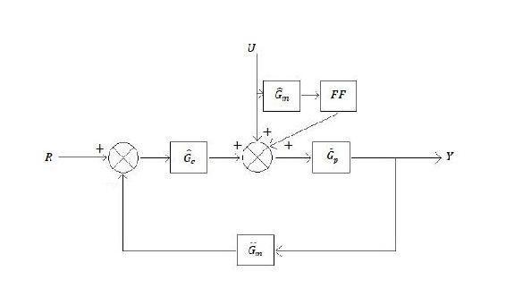
The perfect feed-forward controller is the inverse of the process operator, \(\hat{G}_{P}^{-1}\)
For example:
\[\hat{G}_{P}^{-1}=K_{P}\left(\tau \frac{\delta}{\delta t}+1\right)=\hat{G}_{F F} \nonumber \]
In General:
\[\hat{G}_{P}^{-1} Y=\left(U+\hat{G}_{F F}U\right)+\hat{G}_{C}(R-Y) \nonumber \]
(in the language of operator or state space).
Feed-Forward Control
The objective of feed-forward control is to measure disturbances and compensate for them before the controlled variable deviates from the setpoint. Feed-forward control basically involves a control equation which has certain corrective terms which account for predicted disturbances entering the system. The equation is only effective for gains in a steady state process. Dynamic compensation should be used in the control equation if there are any dynamic deviations with the process response to the control action. This dynamic compensation ability will be discussed further in the next section.
One form of a feed-forward control would be a Derivative (D) control which calculates the change in error and compensates proportionately. But a D-control can’t perform by itself and usually requires working in conjunction with a Proportional (P) or Proportional Integral (PI) control. More information can be found in the PID Intro article.
Simulated below is a typical shell and tube heat exchanger which heats up liquid water using steam.
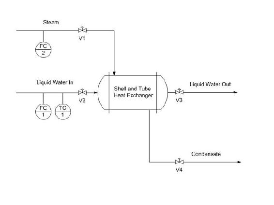
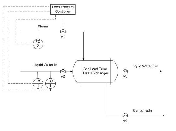
Adding a feed-forward control into the system manipulates the amount of steam required to compensate for the varying amounts of liquid feed coming in.
Overall heat balance:
Heat into the system is equal to the heat leaving the system.
Heat gained by liquid:
\[q_{\text {out}}=m_{l} C_{p}\left(T_{2}-T_{1}\right) \label{1} \]
where:
 -- mass flow rate of the liquid
 -- the heat capacity of the liquid
 -- the input temperature of the liquid
 -- the desired temperature setpoint for the liquid
Heat lost by steam:
\[q_{i n}=m_{s} \lambda \label{2} \]
where:
 -- heat of vaporization
 -- mass flow rate of the steam
Therefore:
\[m_{s}=\frac{C_{p}}{\lambda} m_{l}\left(T_{2}-T_{1}\right) \label{3} \]
To compensate for a deviation from the desired inlet temperature of the liquid water, the amount of steam must be adjusted. Equation (3) acts as the control equation for the feed-forward controller. This controller actuates the inlet valve of the steam and acquires temperature and flow rate data from the inlet streams. Based on the desired temperature setpoint, T2, and the actual input temperature, T1, we can use this equation to calculate the mass flow rate of the steam required to compensate for the temperature deviation.
Accounting for System Non-Idealities
Often, one of the most difficult tasks associated with created a functional feed forward controller is determining the necessary equations that govern the system. Even more complexities arise when the system is not, and cannot be treated as, ideal. This is the case with many real and practical systems. There is simply too much heat lost or too many unforeseen effects to safely assume ideal conditions. The pure math of the example above does not account for these effects.
The equations will output a value to a control valve (often in voltage). That voltage will be derived from some previously determined relationship between voltage, valve %open, and steam flow rate. A very simple way to begin managing the issue of non-ideality is by including a "non-ideality constant". This can be an additive or a multiplicative constant that adjusts the voltage output determined by the equations.
- Voltage output is some function of the calculated required steam flow \[V=f\left(m_{s}\right) \nonumber \]
- Voltage output is adjusted by some constant \[V=c_{N} * f\left(m_{s}\right) \nonumber \] or \[V=c_{N}+f\left(m_{s}\right) \nonumber \]
This non-ideality constant \(c_N\) often must be determined by trial. One way to accomplish this is to use manual control to determine the output voltage needed at various inlet conditions. Using the data from the manual trials, and the resulting voltage that your unadjusted feed forward controller would output, it is possible to determine by what factor your feed forward voltage needs to be adjusted. For example, if by manual control you determine that for inlet conditions X the required voltage is 300 mV and your feed forward controller is only outputting 270 mV for conditions X, you need some factor to adjust.
It may also happen that your "non-ideality constant" will not turn out to be constant when you begin to look at the data. In this situation, consider using a linear relationship between the non-ideality factor and some inlet condition or implementing CASE or IF statements covering discrete ranges of inlet conditions and giving different constants.
Dynamic Compensation
Dynamic compensation is a method to account for factors such as lead and lag times when using feed-forward control. For instance, in the example above, when the feed forward controller monitors a temperature decrease in the liquid feed, it will increase the steam flow rate - the manipulated variable - to compensate and thus maintain the temperature of the exiting liquid flow - the controlled variable. However, the steam may enter the heat exchanger faster than the liquid feed and this will cause a transient increase in the controlled variable from the setpoint. In an ideal case the steam and liquid feed would enter the heat exchanger at the same time and no deviation from the set exiting temperature would be observed. Therefore, dynamic compensation involves predicting non-ideal behavior and accounting for it. While perfect feed-forward control is nearly impossible, dynamic compensation is one step closer.
Open Loop System
Feed-forward control is a open loop system. In an open loop system, the controller uses current, or live, information of the system to generate appropriate actions by using predetermined models. The sensor providing the reference command to the closed loop actuator is not an error signal generated from a feedback sensor but a command based on measurements. This is the defining characteristic of an open loop system, in which the controller does not manipulate the system by trying to minimize errors in the controlled variable.
Because a feed-forward controller listens to the system and calculates adjustments without directly knowing how well the controlled variable is behaving (if it does, it is getting feedback), it is open loop in nature. In other words, the controller operates on "faith", that its mathematical models are able to accurately generate responses (valve setting, motor speed, etc.) that lead to expected results. Therefore, it is critical to implement good models in feed-forward systems. This is often the most difficult part of a feed-forward design, as mentioned previously.
However, not all open loop systems are feed-forward. Open loop simply means the system is not getting feedback information, in which the controlled variable tells the controller how well it is doing compared to its set point (i.e. error). Feed-forward control, on the other hand, takes an extra step by using non-feedback information to produce predictive actions.
This simple open loop system is an example of a open loop system that is not feed-forward. The controller simply takes the current state of the controlled variable to generate a valve setting. It is not getting a feedback, because the product temperature is not compared to a set pont. It is not feed-forward either, because there is no mechanism that produces actions that may yield expected results in the future.
Feed-forward applications
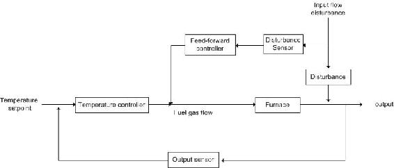
Feed-forward control is used in many chemical engineering applications. These include heat exchangers, CSTRs, distillation columns and many other applications. A typical furnace, shown below, is heating up an input fluid using fuel gas.
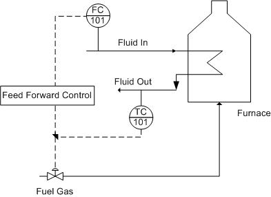
One possible disturbance is the flow rate of the incoming fluid. For example: If the fluid input rate was increased by 10%, then the required heat duty should also be increased by approximately 10%. This feed-forward control strategy immediately changes the fuel gas flow rate and therefore the heat duty. The performance of feed-forward controls is limited by model uncertainty, and in practice feed-forward control is combined with feedback control in order to ensure better control of the system. Feed-forward control will compensate for fluid input disturbances while feedback control will compensate for other disturbances—such as the fuel gas flow rate or the temperature of the furnace—and model uncertainty. This system can also be represented by the following block diagram.
Pros & Cons of Feed-Forward Control
Different applications require different types of control strategies. Sometimes feed-forward solutions are required for proper system control; sometimes only feedback solutions are necessary. Feedback systems don’t always maintain the setpoint as well because of the lag that comes with waiting for the disturbance to propagate through the system. As a result, many control systems use a combination of feed-forward and feedback strategies, such as PID controllers. PID controllers use the Proportional-Integral control for feedback and the Derivative control for feed-forward control. This forms a system with multiple loops, otherwise known as a cascading system. A critical advantage of running both forward and backward controls is that the system is still somewhat able to adjust a variable if one mechanism fails since the two loops use different sensors. As a result, PID controllers are great for controlling processes, however, they require a number of equations to determine feed-forward and feedback correction.
Feed-forward systems work by checking the conditions of an incoming stream and adjusting it before the system is adversely affected. If the controller is told the traits of an acceptable incoming stream, then it can compare that standard to whatever is coming down the pipe. The feed-forward controller can look at this error and send a corrective signal to the automatic valve responsible for that pipe (or any other control device). In order to have this kind of predictive ability, the controller must have explicitly defined equations that account for the effects of a disturbance on the system. In addition, these equations must also then prescribe action to counter-act the disturbance. This can become even more difficult when there are several incoming stream traits that are being observed. When there are multiple inputs, the feed-forward system will require non-linear equations, leading to the development of neural networks.
Neural networks are based on “neurons”, which are representations of non-linear equations. This concept is based on the brain's use of neurons to process and transmit information. The neuron is actually comprised of a set of sigmoidal equations relating inputs to outputs. Sigmoid functions are non-linear equations that take inputs and apply constants, or weights, to transform the value to make an output. Below is a picture that illustrates the function that these neurons serve.
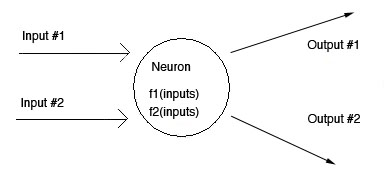
The picture above shows a multiple input-output system. Most feed-forward systems have to deal with more than one input.
Neurons can be “connected” in ways that allow the inputs to be transformed any number of times. Neurons that are connected indicate that one sigmoidal function's output becomes the input of another one. Although the concept of neurons is easily understandable, the difficulty lies in the potential complexity of real systems. For example: the number and type of inputs go to which neurons, the initial weights be, the number of neurons needed, etc. As you can see, there are a lot of design questions that make developing the neural network difficult.
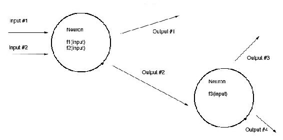
Coupled with an expected set of upstream conditions, the feed-forward system can continually adjust the method it uses to control an output variable. The system is capable of doing this by measuring sensor inputs coming into the controller, using neurons to transform the data, and comparing the resulting output(s) to a set of known or desired outputs. If the actual output is different from the desired output, the weights are altered in some fashion and the process repeats until convergence is achieved. This is how a controller is able to "learn". Learning is just discovering the weighting factors that allow the transformed ouputs to match the desired outputs.
The following table shows a list of feed-forward pros and cons:
| Feed-Forward Pros | Feed-Forward Cons |
|---|---|
|
|
A CSTR with a given volume with heat-exchange capability has a coolant water system to maintain a specific system temperature (368K). To maintain this temperature, the flow of coolant water oscillates. Let a temperature disturbance of 100K be introduced over a period of 10 minutes. For this simulation, the Excel spreadsheet from PID-Tuning Optimization was used to create feed-forward and feed-backward data. In the following plot, observe the difference between using feed-forward control versus feed-backward control in an example.
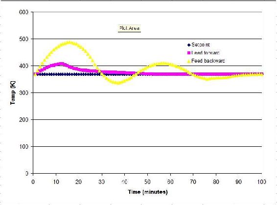
As shown, the feed-forward strategy works more effectively than the feed-backward strategy at nullifying the disturbance (over the time frame). The temperatures reached in feedback mode vary more than the ones seen in feed-forward mode. However, the controller response is solely defined by the parameters used in the Excel spreadsheet. If one assumes that the PID parameters used by the PID-optimization group were optimized, then we can say feed-forward would be the best option here.
This section provides an outline of the different steps for designing a feed-forward control strategy. The steps pay close attention to designing a feed-forward controller where there are multiple disturbances. Feed-forward design can be broken down into eight steps (Corripio,1990).
- Step 1. State the control objective. This step includes defining which variable needs to be controlled and what the set point is. The setpoint should be adjustable by the operator.
- Step 2. List the possible measured disturbances. This step includes identifying which disturbances are easily measured and how fast each disturbance should be expected to vary.
- Step 3. State which variable is going to be manipulated by the feed-forward controller.
- Step 4. The feed-forward controller consists of two parts: steady-state and dynamic compensators. Develop the steady-state compensator first. The compensator should be an equation where the manipulated variable, identified in step 3, can be calculated from the measured disturbances, identified in step 2, and the control objective (set point), identified in step 1.
- Step 5. Reevaluate the list of disturbances. The effect of a disturbance on the controlled variable can be calculated from the equation. Three criteria will be used to determine which disturbance the feed-forward controller will correct: the effect the disturbance has on the controlled variable, the frequency and magnitude of variation, and the capital cost and maintenance of the sensor.
- Step 6. Introduce the feedback compensation. This depends on the physical significance assigned to the feedback signal.
- Step 7. Decide whether dynamic compensation, lead/lag, and/or dead time is required, and decide how to introduce it to the design.
- Step 8. Draw the instrumentation diagram from the feed forward control strategy. The details of the diagram depend largely on the control system being used.
For the first example, a water stream enters an evaporator. A discrete amount of the water stream is to be evaporated. Below is the design diagram for the evaporator. The incoming stream is being used as the input to the feed forward control box.
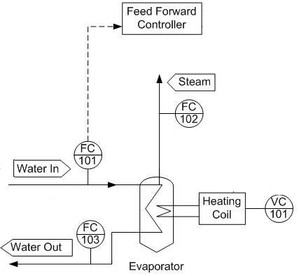
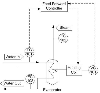
Determine what additional input will be needed to regulate the amount of steam produced and draw this on the design diagram.
Solution
By regulating the heating coil, we can regulate how much water will boil off in accordance with any change of the feed stream.
For the second example, a particular process liquid from a previous reaction will be heated before proceeding to the next phase of reactions. A shell and tube heat exchanger has been installed for this purpose with steam providing the heat duty. A feedback controller is used to control the output temperature of the process liquid stream, but the flowrate and the temperature of the input liquid stream vary too much for the feedback controller to be effective.
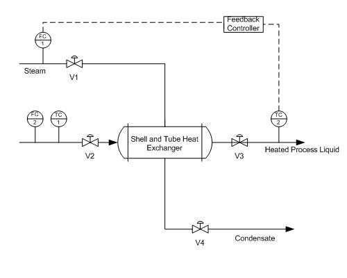
What sort of controller would be appropriate in addition to the feedback controller to account for the deviations of the input liquid stream? How would this controller be implemented? For simplicity it is assumed that all the steam condenses.
Solution
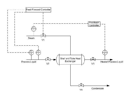
The solution is to implement a feed-forward controller that gathers the input temperature and flowrate data from TC1 and FC2 and adjusts the steam valve V1 in order to account for any deviation that may occur in the input liquid stream. This sort of feedback feed-forward combination is a typical setup for the majority of control systems. The feed-forward controller accounts for any upstream disturbances while the feedback controller accounts for the disturbances within the system.
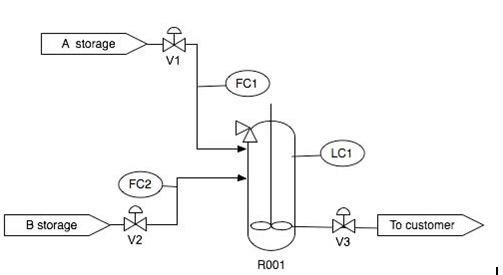
Using the P&ID shown below, write out the feed-forward controller expressions for v3. List any assumptions used in your controller expression.
Solution
To maintain LC1 by measuring FC1 and FC2 and preemptively adjust v3, we must use the controller expression below.
\[v_{3}=k_{\text {valves}}(F C 1+F C 2) \nonumber \]
The controller expression above assumes that the valve is linear. Also, it assumes that FC1, FC2, and the model are infinitely accurate.
References
- Svrcek, William Y., Mahoney, Donald P. & Young, Brett R. (2006). A Real-Time Approach to Process Control. John Wiley & Sons, Ltd.
- Astrom, Karl J. & Hagglund, Tore (1998). Advanced PID Control. Automatic Tuning of PID Controllers. The Instrumentation Systems and Automation Society.
- Smith, Carlos A. & Corripio Armando B. (1997). Principles and Practice of Automatic Process Control. John Wiley & Sons, Inc.
Contributors
Authors: Anwar Stephens, Christopher Garcia, Winardi Kusumaatmaja, Meng Yang Ng


