13.11: Comparisons of two means

Last updated
Save as PDF

Page ID: 22532

Daniel Katzman, Jessica Moreno, Jason Noelanders, & Mark Winston-Galant
University of Michigan

$ \newcommand{\vecs}[1]{\overset { \scriptstyle \rightharpoonup} {\mathbf{#1}} } $

$ \newcommand{\vecd}[1]{\overset{-\!-\!\rightharpoonup}{\vphantom{a}\smash {#1}}} $

$ \newcommand{\id}{\mathrm{id}}$ $ \newcommand{\Span}{\mathrm{span}}$

( \newcommand{\kernel}{\mathrm{null}\,}\) $ \newcommand{\range}{\mathrm{range}\,}$

$ \newcommand{\RealPart}{\mathrm{Re}}$ $ \newcommand{\ImaginaryPart}{\mathrm{Im}}$

$ \newcommand{\Argument}{\mathrm{Arg}}$ $ \newcommand{\norm}[1]{\| #1 \|}$

$ \newcommand{\inner}[2]{\langle #1, #2 \rangle}$

$ \newcommand{\Span}{\mathrm{span}}$

$ \newcommand{\id}{\mathrm{id}}$

$ \newcommand{\Span}{\mathrm{span}}$

$ \newcommand{\kernel}{\mathrm{null}\,}$

$ \newcommand{\range}{\mathrm{range}\,}$

$ \newcommand{\RealPart}{\mathrm{Re}}$

$ \newcommand{\ImaginaryPart}{\mathrm{Im}}$

$ \newcommand{\Argument}{\mathrm{Arg}}$

$ \newcommand{\norm}[1]{\| #1 \|}$

$ \newcommand{\inner}[2]{\langle #1, #2 \rangle}$

$ \newcommand{\Span}{\mathrm{span}}$ $ \newcommand{\AA}{\unicode[.8,0]{x212B}}$

$ \newcommand{\vectorA}[1]{\vec{#1}} % arrow$

$ \newcommand{\vectorAt}[1]{\vec{\text{#1}}} % arrow$

$ \newcommand{\vectorB}[1]{\overset { \scriptstyle \rightharpoonup} {\mathbf{#1}} } $

$ \newcommand{\vectorC}[1]{\textbf{#1}} $

$ \newcommand{\vectorD}[1]{\overrightarrow{#1}} $

$ \newcommand{\vectorDt}[1]{\overrightarrow{\text{#1}}} $

$ \newcommand{\vectE}[1]{\overset{-\!-\!\rightharpoonup}{\vphantom{a}\smash{\mathbf {#1}}}} $

$ \newcommand{\vecs}[1]{\overset { \scriptstyle \rightharpoonup} {\mathbf{#1}} } $

$ \newcommand{\vecd}[1]{\overset{-\!-\!\rightharpoonup}{\vphantom{a}\smash {#1}}} $

$\newcommand{\avec}{\mathbf a}$ $\newcommand{\bvec}{\mathbf b}$ $\newcommand{\cvec}{\mathbf c}$ $\newcommand{\dvec}{\mathbf d}$ $\newcommand{\dtil}{\widetilde{\mathbf d}}$ $\newcommand{\evec}{\mathbf e}$ $\newcommand{\fvec}{\mathbf f}$ $\newcommand{\nvec}{\mathbf n}$ $\newcommand{\pvec}{\mathbf p}$ $\newcommand{\qvec}{\mathbf q}$ $\newcommand{\svec}{\mathbf s}$ $\newcommand{\tvec}{\mathbf t}$ $\newcommand{\uvec}{\mathbf u}$ $\newcommand{\vvec}{\mathbf v}$ $\newcommand{\wvec}{\mathbf w}$ $\newcommand{\xvec}{\mathbf x}$ $\newcommand{\yvec}{\mathbf y}$ $\newcommand{\zvec}{\mathbf z}$ $\newcommand{\rvec}{\mathbf r}$ $\newcommand{\mvec}{\mathbf m}$ $\newcommand{\zerovec}{\mathbf 0}$ $\newcommand{\onevec}{\mathbf 1}$ $\newcommand{\real}{\mathbb R}$ $\newcommand{\twovec}[2]{\left[\begin{array}{r}#1 \\ #2 \end{array}\right]}$ $\newcommand{\ctwovec}[2]{\left[\begin{array}{c}#1 \\ #2 \end{array}\right]}$ $\newcommand{\threevec}[3]{\left[\begin{array}{r}#1 \\ #2 \\ #3 \end{array}\right]}$ $\newcommand{\cthreevec}[3]{\left[\begin{array}{c}#1 \\ #2 \\ #3 \end{array}\right]}$ $\newcommand{\fourvec}[4]{\left[\begin{array}{r}#1 \\ #2 \\ #3 \\ #4 \end{array}\right]}$ $\newcommand{\cfourvec}[4]{\left[\begin{array}{c}#1 \\ #2 \\ #3 \\ #4 \end{array}\right]}$ $\newcommand{\fivevec}[5]{\left[\begin{array}{r}#1 \\ #2 \\ #3 \\ #4 \\ #5 \\ \end{array}\right]}$ $\newcommand{\cfivevec}[5]{\left[\begin{array}{c}#1 \\ #2 \\ #3 \\ #4 \\ #5 \\ \end{array}\right]}$ $\newcommand{\mattwo}[4]{\left[\begin{array}{rr}#1 \amp #2 \\ #3 \amp #4 \\ \end{array}\right]}$ $\newcommand{\laspan}[1]{\text{Span}\{#1\}}$ $\newcommand{\bcal}{\cal B}$ $\newcommand{\ccal}{\cal C}$ $\newcommand{\scal}{\cal S}$ $\newcommand{\wcal}{\cal W}$ $\newcommand{\ecal}{\cal E}$ $\newcommand{\coords}[2]{\left\{#1\right\}_{#2}}$ $\newcommand{\gray}[1]{\color{gray}{#1}}$ $\newcommand{\lgray}[1]{\color{lightgray}{#1}}$ $\newcommand{\rank}{\operatorname{rank}}$ $\newcommand{\row}{\text{Row}}$ $\newcommand{\col}{\text{Col}}$ $\renewcommand{\row}{\text{Row}}$ $\newcommand{\nul}{\text{Nul}}$ $\newcommand{\var}{\text{Var}}$ $\newcommand{\corr}{\text{corr}}$ $\newcommand{\len}[1]{\left|#1\right|}$ $\newcommand{\bbar}{\overline{\bvec}}$ $\newcommand{\bhat}{\widehat{\bvec}}$ $\newcommand{\bperp}{\bvec^\perp}$ $\newcommand{\xhat}{\widehat{\xvec}}$ $\newcommand{\vhat}{\widehat{\vvec}}$ $\newcommand{\uhat}{\widehat{\uvec}}$ $\newcommand{\what}{\widehat{\wvec}}$ $\newcommand{\Sighat}{\widehat{\Sigma}}$ $\newcommand{\lt}{<}$ $\newcommand{\gt}{>}$ $\newcommand{\amp}{&}$ $\definecolor{fillinmathshade}{gray}{0.9}$

Engineers often must compare data sets to determine whether the results of their analyses are statistically equivalent. A sensor outputs a series of values and the engineer must both determine whether the sensor is precise and whether the values are accurate according to a standard. To make this evaluation, statistical methods are used. One method compares the probability distributions and another uses the Students t-test on two data sets. Microsoft Excel also has functions that perform the t-test that output a fractional probability to evaluate the null hypothesis (Basic Statistics).

Distributions

General Distributions

Distributions are governed by the probability density function:

\[f(x)=\frac{1}{\sigma \sqrt{2 \pi}} \exp \left(-\frac{1}{2}\left(\frac{x-\mu}{\sigma}\right)^{2}\right) \nonumber \]

where

$\sigma$ is the standard deviation of a data set
$\sigma$ is the mean of the data set
$\,$ is the input value

This equation gives a typical bell curve. Changing $\sigma$ will alter the shape of the curve, as shown in the graph below.

Changing $\mu$ will shift the curve along the x-axis, as shown below.

Changing both variables will have a result similar to the graph below.

For a more in-depth look at distributions, go to (Distributions).

Overlapping Distributions

The overlap between two distribution curves helps determine the probability of the two data sets being from the same distribution. The probability value increases as overlapping increases. The overlap is shown as the purple region in the graph below.

Comparison of Two Means

Probability

The similarity of two data sets can be determined by finding the probability of overlap. This is illustrated by the following equation:

\[P(\text { overlap })=\int_{-\infty}^{\infty} \min \left\{\begin{array}{l}
p_{s}\left(k \mid \theta_{s}\right) \\
p_{o}\left(k \mid \theta_{0}\right)
\end{array}\right. \nonumber \]

The functions contained within the integral are the probability distributions of each respective data set. The equation sums the lesser probability distribution from each data set. After using this equation, the solution will be a value with a range between 0 and 1 indicating the magnitude of overlapping probability. A value of 0 demonstrates that the two data sets do not overlap at all. A value of 1 demonstrates that the two data sets completely overlap. Values between 0 and 1 give the extent of overlap between the two data sets. This probability is not the same as the confidence interval that can be computed with t-tests.

Student's T-Test

The Student’s t-test is extremely useful for comparing two means. There are various versions of the student t-test, depending on the context of the problem. Generally, the test quantifies the signal to noise ratio - where the signal is the difference of means and the noise is a function of the error around the means. If the signal is large and the noise is small, one can be more confident that the difference between the means is "real" or significant. To prove a significant difference, we need to disprove the null hypothesis. The "null hypothesis" (Ho) is that there is no difference between the two means. If we are able to disprove the "null hypothesis" then we will be able to say that the two groups are statistically different within a known level of confidence.

The extremities at either ends of a probability distribution are referred to as the "tails" of the distribution. The assessment of the significance of a calculated t-value will depend upon whether or not both tails of the distribution need to be considered. This will depend on the form of the null hypothesis. If your null hypothesis is an equality, then the case where one mean is larger and smaller must be considered; i.e. only one tail of the distribution should be accounted for. Conversely, if the null hypothesis is an inequality, then you are only concerned with the domain of values for a mean either less than or greater than the other mean; i.e. both tails of the distribution should be accounted for.

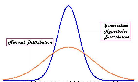
More Info: the student t-distribution

The t-distribution is the resulting probability distribution with a small sample population. This distribution is the basis for the t-test, in order to find the statistical significance between two means of data. This distribution is in the form of a generalised hyperbolic function (Which goes into details that would only clutter here. For more information, the Wikipedia site holds a lot of information on the subject: en.Wikipedia.org/wiki/Generalised_hyperbolic_distribution).

The t-distribution is commonly used when the standard deviation is unknown, or cannot be known (ie: a very small population set). When the data sets are large, or a standard deviation is assumed, the t-distribution is not very useful for a statistical analysis, and other methods of analysis should be used. An example of the t-distribution can be seen below:

Comparing Two Unknown True Means when Sample Standard Deviations are approximately Equal

The first accepted assumption is that when two sample means are being compared, the standard deviations are approximately equal. This method requires the average, standard deviation, and the number of measurements taken for each data set. The deviations are then pooled into one standard deviation. The equation for this t-test is as follows:

\[t=\frac{\text { Signal }}{\text { Noise }}=\frac{\bar{x}_{1}-\bar{x}_{2}}{S_{\text {pooled }}} \sqrt{\frac{n_{1} n_{2}}{n_{1}+n_{2}}} \nonumber \]

where:

\[S_{\text {pooled }}=\sqrt{\frac{s_{1}^{2}\left(n_{1}-1\right)+s_{2}^{2}\left(n_{2}-1\right)}{n_{1}+n_{2}-2}} \nonumber \]

where:

$\overline{x}_1 $ is the average of the first data set
$\overline{x}_2 $ is the average of the second data set
$n_1$ is the number of measurements in the first data set
$n_2$ is the number of measurements in the second data set
$s_1$ is the standard deviation of the first data set
\(s_2) is the standard deviation of the second data set
$t$ is a result of the t-test; it relates to values from the Student's t-distribution

Also note that the variance is defined as the square of the standard deviation.

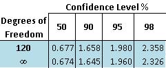
Using t-distribution tables (sample shown below), the confidence level for the two means can then be determined. This confidence level determines whether the two means are significantly different. The confidence level can be found with the degrees of freedom for the measurements and the t-value computed above. The degree of freedom is equal to two less than the total number of measurements from the two data sets, as shown below:

\[D O F=n_{1}+n_{2}-2 \nonumber \]

The following table is an image of a t value table, which can also be found (here):

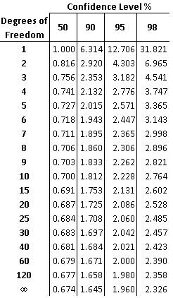
For example, if you had two data sets totaling 10 measurements and you calculated a t-value of 2.305 the confidence level would be 95%. This means that there is a 95% chance that the two data sets are statistically different and only a 5% chance that the two data sets are statistically similar. Also, degrees of freedom between the values listed on the table can be found by interpolating between those two values.

Note that there are some drawbacks when evaluating two means to see if they are significant or not. This problem mainly stems from the standard deviation. If say a set of values has a certain mean x, but the standard deviation was high due to the fact that some numbers in may have been greatly out of the range of the mean. This standard deviation may imply, from the student's t-test, that the mean x is significantly different from the mean of another set of data, when in actuality it may not seem that different. Hence, this must be taken into account when comparing two means using the student's t-test.

Comparing Two Unknown True Means (μ₁ = ? and μ₂ = ?) with Known True Unequal Standard Deviations (\[\\sigma_1 \neq \sigma_2 \nonumber \])

The z-test is used when the difference between a sample mean and the population mean is large enough to be statistically significant. The t-test and z-test are essentially the same but in the z-test the actual population means ( $mu\,$ ) and standard deviations( $sigma\,$ ) are known. Since the estimate for difference in standard deviation used here is biased, two sample z-tests are rarely used.

The two sample z-statistic is described by:

\[z=\frac{\text { Signal }}{\text { Noise }}=\frac{\bar{x}_{1}-\bar{x}_{2}}{\sqrt{\frac{\sigma_{1}^{2}}{n_{1}}+\frac{\sigma_{2}^{2}}{n_{2}}}} \nonumber \]

where:

$\overline{x}_1 $ is the average of the first data set
$\overline{x}_2 $ is the average of the second data set
$n_1$ is the number of measurements in the first data set
$n_2$ is the number of measurements in the second data set
$\sigma_1 $ is the known standard deviation of the first population
$\sigma_2 $ is the known standard deviation of the second population

A different table is used to look up the probability of significance, please refer to Z-score table. If p < 0.05 (using a 95% confidence interval), we can declare a significant difference exists. The p-value is the probability that the observed difference between the means is caused by sampling variation, or the probability that these two samples came from the same population.

Comparing Two Unknown True Means (μ₁ = ? and μ₂ = ?) with Unknown True Standard Deviations (σ₁ = ? and σ₂ = ?)

This is known as the two sample t-statistic, which is used in statistical inference for comparing the means of two independent, normally distributed populations with unknown true standard deviations. The two sample t-statistic is described by:

\[t=\frac{\text { Signal }}{\text { Noise }}=\frac{\bar{x}_{1}-\bar{x}_{2}}{\sqrt{\frac{s_{1}^{2}}{n_{1}}+\frac{s_{2}^{2}}{n_{2}}}} \nonumber \]

Where:

\[\\overline{x}_1 \nonumber \]is the average of the first data set
\[\\overline{x}_2 \nonumber \]is the average of the second data set
$n_1 \,$ is the number of measurements in the first data set
$n_2 \,$ is the number of measurements in the second data set
$s_1 \,$ is the standard deviation of the first data set
$s_2 \,$ is the standard deviation of the second data set

Comparing the Mean of Differences for Paired Data

This is used in statistical analysis for the case where a single mean of a population occurs when two quantitative variables are collected in pairs, and the information we desire from these pairs is the difference between the two variables.

Two examples of paired data:

Each unit is measured twice. The two measurements of the same data are taken under varied conditions.
Similar units are paired prior to the experiment or run. During the experiment or run each unit is placed into different conditions.

The mean of differences t-statistic is described by:

\[t=\frac{\bar{d}}{\frac{s_{d}}{\sqrt{n}}} \nonumber \]

where:

$\overline{d} $ is the the mean of the differences for a sample of the two measurements
$s_d \,$ is the standard deviation of the sampled differences
$n \,$ is the number of measurements in the sample

Summary of Two Sample Mean Tests

wo sample mean tests.jpg

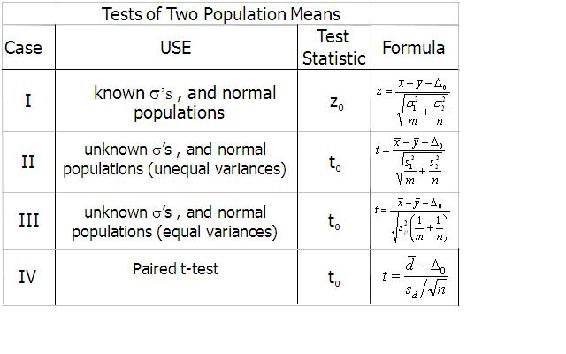
Excel Method

Instead of using the t-distribution tables to interpolate values, it is often easier to use built-in tools in Excel. The following three functions can be used for most of the common situations encountered when comparing two means:

The TDIST function is useful when you have calculated a t-value and you want to know the probability that the t-value is significant.
The TINV function is useful when you know the probability of significance you are interested in, and you desire the t-value (essentially the reverse of the TDIST function). This is helpful if you are designing an experiment and would like to determine the number of experimental runs needed to test for the difference of two means.
The TTEST function is useful if you have two sets of data and you would like to know the probability that the mean of the two data sets are significantly different.

TDIST Function

The TDIST function has the syntax "=TDIST(x,deg_freedom,tails)"

Where:

x is the t-value of the statistic
deg_freedom is the number of degrees of freedom of the t-statistic. For comparing sample means $\overline{x}_o$ and $\overline{x}_s$ , with sample sizes $n_o \,$ and $n_s \,$ respectively, has 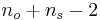$n_o + n_s - 2 \,$ degrees of freedom.
tails is the number of tails to be summed for probability. If null hypothesis is an equality, 2 tails will be used. If the null hypothesis is an inequality, 1 tail will be used.

The output of the function is the fractional probability of the Students t-distribution. For example, if the function returned a value of 0.05, this would correspond to a 95% or equivalently (1 - 0.05) confidence level for rejecting the null hypothesis.

TINV Function

The TINV function has the syntax "=TINV(probalility, deg_freedom)"

where:

probability is the fractional probability of the Students t-distribution. This is identical to the output of the "TDIST" function.
deg_freedom is the number of degrees of freedom of the t-statistic. For comparing sample means $\overline{x}_o$ and $\overline{x}_s$ , with sample sizes $n_o \,$ and $n_s \,$ respectively, has $n_o + n_s - 2 \,$ degrees of freedom.

The output of the function is the t-value of the Student's t-distribution.

TTEST Function

The TTEST function has the syntax "=TTEST(array 1, array 2, tails, type)"

where:

array 1 is the first data set
array 2 is the second data set
tails is the number of tails to be summed for probability (1 or 2). If null hypothesis is an equality 2 tails will be used, if the null hypothesis is an inequality 1 tail will be used.
type is the type of t-test to be performed the values that correspond to each type of test are listed below.

If type equals | This test is performed 1 | Paired 2 | Two-sample equal variance (homoscedastic) 3 | Two-sample unequal variance (heteroscedastic)

For our purposes we will only be concerned with type = 3. This corresponds to unequal variance (independent data sets). The other two types are useful and may prove interesting for the curious, but are beyond our scope.

Alternatively if you are not fond of Excel, a website located here will do the TTEST calculation for you.

The output of the function is the fractional probability of the Student's t-distribution. For example, if the function returned a value of 0.05, this would correspond to a 95% or equivalently (1 - 0.05) confidence level for rejecting the null hypothesis.

This function is very useful when the data-sets of the two means to be compared are known.

Worked out Example 1

You are a product quality engineer at a company that manufactures powdered laundry detergent in 100 ounce boxes. You are in charge of determining whether the product meets the specifications the company promises the customer. In the past, 100 samples $\left(n_o \right)$ of the process established normal process conditions. The data is given below. Note that weighing samples using an imprecise scale does not affect your results. Also assume that the standard deviations are close enough to pool them.

You randomly sample 25 $\left( n_s \right )$ of the products and you get the following data:

The data can also be found in the first tab of this Excel file: Data File

Is the process running significantly different from normal with 95% confidence? In this example, do not use built-in Excel functions.

Solution

Using the data, the normal process produces an average $\left( \overline{x}_o \right )$ product mass of 102.37 and a variance $\left( s_o^2 \right )$ of 3.17.

The sample has an average mass $\left ( \overline{x}_s \right )$ of 100.00 with a variance $\left ( s_s^2 \right )$ of 4.00.

These were calculated using the AVERAGE function and VAR function in Excel. See the second tab of this Excel file for further explanation: Example 1

The null hypothesis is that the means are identical and the difference between the two means is due purely to chance.

Using the t-test:

\[t=\frac{\bar{x}_{o}-\bar{x}_{s}}{\sqrt{\frac{s_{o}^{2}\left(n_{o}-1\right)+s_{s}^{2}\left(n_{s}-1\right)}{n_{o}+n_{s}-2}}} \sqrt{\frac{n_{o} n_{s}}{n_{o}+n_{s}}} \nonumber \]

\[t=\frac{102-100}{\sqrt{\frac{3(100-1)+4(25-1)}{100+25-2}}} \sqrt{\frac{25 * 100}{25+100}}=5.00 \nonumber \]

Looking at the table that is reprinted below for reference:

The number of degrees of freedom is:

$DOF = n_o + n_s - 2 \,$

$DOF = 25 + 100 - 2 = 123 \,$

The t-value corresponding to 95% confidence level at 123 degrees of freedom is between 1.960 and 1.980. Since the calculated t-value, 5.00, is much greater than 1.980, the null hypothesis is rejected at the 95% confidence level.

We conclude that the two means are significantly different. Thus, the process is not running normally and it is time to troubleshoot to find the problems occurring in the system.

Worked out Example 2

Same problem as "Worked Out Example 1." Instead, use the TTEST function in Excel.

Solution

The solution can also be seen in the third tab of this Excel file: Example 2

Using the TTEST function, with tails = 2 and test type = 3, the function gives a T-test value of $4.78 x 10^{-6}\,$ .

Since $4.78 x 10^{-6}\,$ is less than 0.05 (from our 95% confidence level) we can once again conclude that we can reject the null hypothesis.

Exercise $\PageIndex{1}$

If there are two sets of data, one with 15 measurements and another with 47 measurements, how many degrees of freedom would you enter in the Excel functions?

Answer

The number of degrees of freedom is calculated as follows:

$DOF = n_1 + n_2 - 2 \,$

where n₁ is the number of measurements in the first data set and n₂ is the number of measurements in the second data set.

Therefore,

$DOF = 15 + 47 - 2 = 60 \,$

the answer is d.

Exercise $\PageIndex{2}$

What does the statement "Accurate within 95% confidence" mean?

The average of the data set is statistically equal to the true value within 95%
The value is the average plus or minus 95%
The average is statistically equal to the true value within 5%

Answer: c

References

"Comparison of Two Means." State.Yale.Edu. Yale. 19 Nov. 2006 <http://www.stat.yale.edu/Courses/1997-98/101/meancomp.htm>.
Excel Help File. Microsoft 2006.
Harris, Daniel C. Exploring Chemical Analysis. 3rd ed. New York: W. H. Freeman and Company, 2005. 77-151.
Woolf, Peter, et al. Statistics and Probability Primer for Computational Biologists. Massachusetts Institute of Technology. BE 490/Bio 7.91. Spring 2004. 52-68.
"Z-test." Wikipedia. en.Wikipedia.org/wiki/Z-test

Search

Text Color

Text Size

Margin Size

Font Type

Exercise \(\PageIndex{1}\)

Exercise \(\PageIndex{2}\)