2.1: System Poles and Zeros
- Page ID
- 24393

System Poles and Zeros
The transfer function, \(G(s)\), is a rational function in the Laplace transform variable, \(s\). It is expressed as the ratio of the numerator and the denominator polynomials, i.e., \(G(s)=\frac{n(s)}{d(s)}\).
The roots of the numerator polynomial, \(n(s)\), define system zeros, i.e., those frequencies at which the system response is zero. Thus, \(z_0\) is a zero of the transfer function if \(G\left(z_0\right)=0.\)
The roots of the denominator polynomial, \(d(s)\), define system poles, i.e., those frequencies at which the system response is infinite. Thus, \(p_0\) is a pole of the transfer function if \(G\left(p_0\right)=\infty .\)
The poles and zeros of first and second-order system models are described below.
First-Order System
A first-order system has a generic ODE description: \(\tau \dot{y}\left(t\right)+y\left(t\right)=u(t)\), where \(u\left(t\right)\) and \(y\left(t\right)\) denote the input and the output, and \(\tau\) is the system time constant. By applying the Laplace transform, a first-order transfer function is obtained as: \[G(s)=\frac{K}{\tau s+1} \nonumber \]
The transfer function has no finite zeros and a single pole located at \(s=-\frac{1}{\tau }\) in the complex plane.
The reduced-order model of a DC motor with voltage input and angular velocity output (Example 1.4.3) is described by the differential equation: \(\tau \dot\omega (t) + \omega(t) = V_a(t)\).
The DC motor has a transfer function: \(G(s)=\frac{K}{\tau_m s+1}\) where \(\tau_m\) is the motor time constant.
For the following parameter values: \(R=1\Omega ,\; L=0.01H,\; J=0.01\; kgm^{2} ,\; b=0.1\; \frac{N-s}{rad} ,\; and\; k_{t} =k_{b} =0.05\), the motor transfer function evaluates as:
\[G(s)=\frac{\omega (s)}{V_{ a} (s)} =\frac{5}{s+10.25}=\frac{0.49}{0.098 s+1} \nonumber \]
The transfer function has a single pole located at: \(s=-10.25\) with associated time constant of \(0.098 sec\).
Second-Order System with an Integrator
A first-order system with an integrator is described by the transfer function:
\[G\left(s\right)=\frac{K}{s(\tau s+1)} \nonumber \]
The system has no finite zeros and has two poles located at \(s=0\) and \(s=-\frac{1}{\tau }\) in the complex plane.
The DC motor modeled in Example 2.1.1 above is used in a position control system where the objective is to maintain a certain shaft angle \(\theta(t)\). The motor equation is given as: \(\tau \ddot\theta(t) + \dot\theta(t) = V_a(t)\); its transfer function is given as: \(G\left(s\right)=\frac{K}{s(\tau s+1)}\).
Using the above parameter values in the reduced-order DC motor model, the system transfer function is given as:
\[G(s)=\frac{\theta (s)}{V_{ a} (s)} =\frac{5}{s(s+10.25)}=\frac{0.49}{s(0.098 s+1)} \nonumber \]
The transfer function has no finite zeros and poles are located at: \(s=0,-10.25\).
Second-Order System with Real Poles
A second-order system with poles located at \(s=-{\sigma }_1,\ -{\sigma }_2\) is described by the transfer function:
\[G\left(s\right)=\frac{1}{\left(s+{\sigma }_1\right)\left(s+{\sigma }_2\right)} \nonumber \]
From Section 1.4, the DC motor transfer function is described as: \[G(s)=\frac{K}{(s+1/\tau _{e} )(s+1/\tau _{m} )} \nonumber \]
Then, system poles are located at: \(s_{1} =-\frac{1}{\tau _{m} }\) and \(s_{2} =-\frac{1}{\tau _{e} }\), where \(\tau_e\) and \(\tau_{m}\) represent the electrical and mechanical time constants of the motor.
For the following parameter values: \(R=1\Omega ,\; L=0.01H,\; J=0.01\; kgm^{2} ,\; b=0.1\; \frac{N-s}{rad} ,\; and\; k_{t} =k_{b} =0.05\), the transfer function from armature voltage to angular velocity is given as:
\[\frac{\omega (s)}{V_{ a} (s)} =\frac{500}{(s+100)(s+10)+25} =\frac{500}{(s+10.28)(s+99.72)} \nonumber \]
The transfer function poles are located at: \(s=-10.28, -99.72\).
The motor time constants are given as: \(\tau _{e} \cong \frac{L}{R}=10 \;ms,\; \tau _ m \cong \frac{J}{b}=100\; ms\).
Second-Order System with Complex Poles
A second-order model with its complex poles located at: \(s=-\sigma \pm j\omega\) is described by the transfer function:
\[G\left(s\right)=\frac{K}{{\left(s+\sigma \right)}^2+{\omega }^2}. \nonumber \]
Equivalently, the second-order transfer function with complex poles is expressed in terms of the damping ratio, \(\zeta\), and the natural frequency, \({\omega }_n\), of the complex poles as:
\[G(s)=\frac{K}{(s+\zeta {\omega }_n)^2+{\omega }^2_n(1-\zeta^2)} \nonumber \]
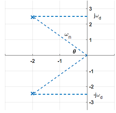
The transfer function poles are located at: \(s_{1,2}=-\zeta {\omega }_n\pm j{\omega }_d\), where \({\omega }_d=\omega_n\sqrt{1-{\zeta }^2}\) (Figure 2.1.1).
As seen from the figure, \({\omega }_n\) equals the magnitude of the complex pole, and \(\zeta =\frac{\sigma }{{\omega }_n}={\cos \theta }\), where \(\theta\) is the angle subtended by the complex pole at the origin.
The damping ratio, \(\zeta\), is a dimensionless quantity that characterizes the decay of the oscillations in the system’s natural response. The damping ratio is bounded as: \(0<\zeta <1\).
- As \(\zeta \to 0\), the complex poles are located close to the imaginary axis at: \(s\cong \pm j{\omega }_n\). The resulting impulse response displays persistent oscillations at system’s natural frequency, \({\omega }_n\).
- As \(\zeta \to 1\), the complex poles are located close to the real axis as \(s_{1,2}\cong -\zeta {\omega }_n\). The resulting impulse response has no oscillations and exponentially decays to zero resembling the response of a first-order system.
A spring–mass–damper system has a transfer function:
\[G(s)=\frac{1}{ms^{2} +bs+k}. \nonumber \]
Its characteristic equation is given as: \(ms^s+bs+k=0\), whose roots are characterized by the sign of the discriminant, \(\Delta =b^{2} -4mk\).
Specifically,
- For \(\Delta >0,\) the system has real poles, located at:
\(s_{1,2} =-\frac{b}{2m} \pm \sqrt{\left(\frac{b}{2m} \right)^{2} -\frac{k}{m} }.\)
- For \(\Delta <0,\) the system has complex poles, located at:
\(s_{1,2} =-\frac{b}{2m} \pm j\sqrt{\frac{k}{m} -\left(\frac{b}{2m} \right)^{2} }.\)
- For \(\Delta=0\), the system has two real and equal poles, located at:
\(s_{1,2} =-\frac{b}{2m}.\)
Next, assume that the mass-spring-damper has the following parameter values: \(m=1, b=k=2\); then, its transfer function is given as: \[G(s)=\frac{1}{ms^2+bs+k}=\frac{1}{s^2+2s+2} \nonumber \]
The transfer function has complex poles located at: \(s=-1\pm j1\).
The complex poles have: \({\omega }_n=\sqrt{2} \frac{rad}{s}, \zeta =\frac{1}{\sqrt{2}}\).
Further, the complex poles have an angle: \(\theta=45^\circ\), and \(\cos45^\circ=\frac{1}{\sqrt{2}}\).