7.2: Pulse Transfer Function

Zero-Order Hold

A zero-order hold (ZOH) reconstructs a piece-wise constant signal from a number sequence and represents a model of the digital-to-analog converter (DAC).

Assuming that the input to the ZOH is a sampled signal, \(r(kT)=\left. r(t)\right|_{t=kT}\), its output is given as:

\[r(t)=r((k-1)T)\quad {\rm for}\quad (k-1)T\le t<kT \nonumber \]

The output of the ZOH to an arbitrary input, \(r\left(kT\right)\), is a staircase reconstruction of the analog signal, \(r(t)\).

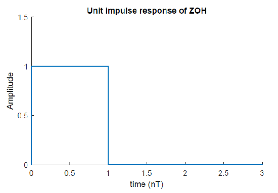
The impulse response of the ZOH is square pulse (Figure 7.2): \(g_{ZOH} (t)=1,\; 0<t<1\).

By applying Laplace transform to the ZOH impulse response, its transfer function is obtained as:

\[G_{{\rm ZO}H} (s)=\frac{1}{s} -\frac{e^{-sT} }{s} =\frac{1-e^{-sT} }{s} \nonumber \]

Further, the frequency response function of the ZOH is given as:

\[G_{\rm ZOH} (\omega )=\frac{1-e^{-j\omega T} }{j\omega } =T\frac{\sin (\omega T/2)\; }{\omega T/2} e^{-j\omega T/2} \nonumber \]

Thus, the frequency response of the ZOH is a \(sinc\) function with a phase delay. When placed in the feedback loop, the added phase from the ZOH reduces the available phase margin, adversely impacting closed-loop stability.

Specifically, let \(\omega _{gc}\) denote the gain crossover frequency; then, the phase margin is reduced by \(\omega _{gc} T/2.\)

The acceptable degradation in the \(\rm PM\) can be used to select the sample time, \(T\). For example, if we want to limit the \(\rm PM\) degradation to \(5^{\circ } \; (0.087\; {\rm r}ad)\), the sampling time may be selected as: \(T\le \frac{0.175}{\omega _{\rm gc} }\).

Figure \(\PageIndex{1}\): Impulse response of the ZOH.

The Pulse Transfer Function

We use \(z\)-transform to obtain a transfer function description of the plant cascaded with the ZOH. The result is the pulse transfer function, \(G(z)\), that is valid at the sampling intervals.

The pulse transfer function of a continuous-time plant, \(G(s)\), is obtained as:

\[G(z)={\rm z}\left\{\frac{1-e^{-sT} }{s} G(s)\right\}=(1-z^{-1} ){\rm z}\left\{\frac{G(s)}{s} \right\} \nonumber \]

where \(z\left\{\frac{G\left(s\right)}{s}\right\}\) denotes the \(z\)-transform of a sequence obtained by sampling \(\int g\left(t\right)dt\).

Example \(\PageIndex{1}\)

Let \(G(s)=\frac{a}{s+a}\); then \(G(z)=(1-z^{-1} )\; {\rm z}\left\{\frac{a}{s(s+a)} \right\}=(1-z^{-1} ){\rm z}\left\{\frac{1}{s} -\frac{1}{s+a} \right\}.\)

By using the \(z\)-transform table, we obtain: \(G(z)=\frac{z-1}{z} \left(\frac{z}{z-1} -\frac{z}{z-e^{-aT} } \right)=\frac{1-e^{-aT} }{z-e^{-aT} } \).

As an example, let \(G(s)=\frac{1}{s+1},\; T=0.2s\). Then, the pulse transfer function is obtained as: \(G(z)=\frac{0.181}{z-0.819}\), or \(G(z)=\frac{1-e^{-0.2} }{z-e^{-0.2} }\).

 

Example \(\PageIndex{2}\)

Let \(G(s)=\frac{a}{s(s+a)}\); then \(G(z)=(1-z^{-1} )\; {\rm z}\left\{\frac{a}{s^{2} (s+a)} \right\}=(1-z^{-1} ){\rm z}\left\{\frac{1}{s^{2} } -\frac{1/a}{s} +\frac{1/a}{s+a} \right\} \).

By using the z-transform table, we obtain: \(G(z)=\frac{z-1}{z} \left[\frac{Tz}{(z-1)^{2} } -\frac{1}{a} \left(\frac{z}{z-1} -\frac{z}{z-e^{-aT} } \right)\right]=\frac{aT(z-e^{-aT} )-(z-1)(1-e^{-aT} )}{a(z-1)(z-e^{-aT} )} \).

As an example, let \(G(s)=\frac{1}{s(s+1)} ,\; T=0.2s;\) then, the pulse transfer function is obtained as: \(G(z)=\frac{0.0187(z+0.936)}{(z-1)(z-0.819)}\).

From the above examples, we observe that:

1. The order of the pulse transfer function, i.e., the degree of the denominator polynomial in\(G(z)\), matches that of the continuous-time transfer function, \(G(s)\).
2. The poles of the pulse transfer function are related to the transfer function poles as: \(z_ i =e^{s_ i T}\).
3. The pulse transfer functions of the second and higher order systems additionally includes finite zeros.

In the MATLAB Control Systems Toolbox, the pulse transfer function is obtained by using the “c2d” command and specifying a sampling time (\(T_s\)). The command is invoked after defining the continuous-time transfer function model.

The choice of the sampling time is guided by the natural frequency of the system. In particular, we may choose \(T_s\ll 1/{\omega }_n\), where \({\omega }_n\) represents the natural frequency.