
4.6: Problems
- Page ID
- 82604
\( \newcommand{\vecs}[1]{\overset { \scriptstyle \rightharpoonup} {\mathbf{#1}} } \)
\( \newcommand{\vecd}[1]{\overset{-\!-\!\rightharpoonup}{\vphantom{a}\smash {#1}}} \)
\( \newcommand{\dsum}{\displaystyle\sum\limits} \)
\( \newcommand{\dint}{\displaystyle\int\limits} \)
\( \newcommand{\dlim}{\displaystyle\lim\limits} \)
\( \newcommand{\id}{\mathrm{id}}\) \( \newcommand{\Span}{\mathrm{span}}\)
( \newcommand{\kernel}{\mathrm{null}\,}\) \( \newcommand{\range}{\mathrm{range}\,}\)
\( \newcommand{\RealPart}{\mathrm{Re}}\) \( \newcommand{\ImaginaryPart}{\mathrm{Im}}\)
\( \newcommand{\Argument}{\mathrm{Arg}}\) \( \newcommand{\norm}[1]{\| #1 \|}\)
\( \newcommand{\inner}[2]{\langle #1, #2 \rangle}\)
\( \newcommand{\Span}{\mathrm{span}}\)
\( \newcommand{\id}{\mathrm{id}}\)
\( \newcommand{\Span}{\mathrm{span}}\)
\( \newcommand{\kernel}{\mathrm{null}\,}\)
\( \newcommand{\range}{\mathrm{range}\,}\)
\( \newcommand{\RealPart}{\mathrm{Re}}\)
\( \newcommand{\ImaginaryPart}{\mathrm{Im}}\)
\( \newcommand{\Argument}{\mathrm{Arg}}\)
\( \newcommand{\norm}[1]{\| #1 \|}\)
\( \newcommand{\inner}[2]{\langle #1, #2 \rangle}\)
\( \newcommand{\Span}{\mathrm{span}}\) \( \newcommand{\AA}{\unicode[.8,0]{x212B}}\)
\( \newcommand{\vectorA}[1]{\vec{#1}} % arrow\)
\( \newcommand{\vectorAt}[1]{\vec{\text{#1}}} % arrow\)
\( \newcommand{\vectorB}[1]{\overset { \scriptstyle \rightharpoonup} {\mathbf{#1}} } \)
\( \newcommand{\vectorC}[1]{\textbf{#1}} \)
\( \newcommand{\vectorD}[1]{\overrightarrow{#1}} \)
\( \newcommand{\vectorDt}[1]{\overrightarrow{\text{#1}}} \)
\( \newcommand{\vectE}[1]{\overset{-\!-\!\rightharpoonup}{\vphantom{a}\smash{\mathbf {#1}}}} \)
\( \newcommand{\vecs}[1]{\overset { \scriptstyle \rightharpoonup} {\mathbf{#1}} } \)
\(\newcommand{\longvect}{\overrightarrow}\)
\( \newcommand{\vecd}[1]{\overset{-\!-\!\rightharpoonup}{\vphantom{a}\smash {#1}}} \)
\(\newcommand{\avec}{\mathbf a}\) \(\newcommand{\bvec}{\mathbf b}\) \(\newcommand{\cvec}{\mathbf c}\) \(\newcommand{\dvec}{\mathbf d}\) \(\newcommand{\dtil}{\widetilde{\mathbf d}}\) \(\newcommand{\evec}{\mathbf e}\) \(\newcommand{\fvec}{\mathbf f}\) \(\newcommand{\nvec}{\mathbf n}\) \(\newcommand{\pvec}{\mathbf p}\) \(\newcommand{\qvec}{\mathbf q}\) \(\newcommand{\svec}{\mathbf s}\) \(\newcommand{\tvec}{\mathbf t}\) \(\newcommand{\uvec}{\mathbf u}\) \(\newcommand{\vvec}{\mathbf v}\) \(\newcommand{\wvec}{\mathbf w}\) \(\newcommand{\xvec}{\mathbf x}\) \(\newcommand{\yvec}{\mathbf y}\) \(\newcommand{\zvec}{\mathbf z}\) \(\newcommand{\rvec}{\mathbf r}\) \(\newcommand{\mvec}{\mathbf m}\) \(\newcommand{\zerovec}{\mathbf 0}\) \(\newcommand{\onevec}{\mathbf 1}\) \(\newcommand{\real}{\mathbb R}\) \(\newcommand{\twovec}[2]{\left[\begin{array}{r}#1 \\ #2 \end{array}\right]}\) \(\newcommand{\ctwovec}[2]{\left[\begin{array}{c}#1 \\ #2 \end{array}\right]}\) \(\newcommand{\threevec}[3]{\left[\begin{array}{r}#1 \\ #2 \\ #3 \end{array}\right]}\) \(\newcommand{\cthreevec}[3]{\left[\begin{array}{c}#1 \\ #2 \\ #3 \end{array}\right]}\) \(\newcommand{\fourvec}[4]{\left[\begin{array}{r}#1 \\ #2 \\ #3 \\ #4 \end{array}\right]}\) \(\newcommand{\cfourvec}[4]{\left[\begin{array}{c}#1 \\ #2 \\ #3 \\ #4 \end{array}\right]}\) \(\newcommand{\fivevec}[5]{\left[\begin{array}{r}#1 \\ #2 \\ #3 \\ #4 \\ #5 \\ \end{array}\right]}\) \(\newcommand{\cfivevec}[5]{\left[\begin{array}{c}#1 \\ #2 \\ #3 \\ #4 \\ #5 \\ \end{array}\right]}\) \(\newcommand{\mattwo}[4]{\left[\begin{array}{rr}#1 \amp #2 \\ #3 \amp #4 \\ \end{array}\right]}\) \(\newcommand{\laspan}[1]{\text{Span}\{#1\}}\) \(\newcommand{\bcal}{\cal B}\) \(\newcommand{\ccal}{\cal C}\) \(\newcommand{\scal}{\cal S}\) \(\newcommand{\wcal}{\cal W}\) \(\newcommand{\ecal}{\cal E}\) \(\newcommand{\coords}[2]{\left\{#1\right\}_{#2}}\) \(\newcommand{\gray}[1]{\color{gray}{#1}}\) \(\newcommand{\lgray}[1]{\color{lightgray}{#1}}\) \(\newcommand{\rank}{\operatorname{rank}}\) \(\newcommand{\row}{\text{Row}}\) \(\newcommand{\col}{\text{Col}}\) \(\renewcommand{\row}{\text{Row}}\) \(\newcommand{\nul}{\text{Nul}}\) \(\newcommand{\var}{\text{Var}}\) \(\newcommand{\corr}{\text{corr}}\) \(\newcommand{\len}[1]{\left|#1\right|}\) \(\newcommand{\bbar}{\overline{\bvec}}\) \(\newcommand{\bhat}{\widehat{\bvec}}\) \(\newcommand{\bperp}{\bvec^\perp}\) \(\newcommand{\xhat}{\widehat{\xvec}}\) \(\newcommand{\vhat}{\widehat{\vvec}}\) \(\newcommand{\uhat}{\widehat{\uvec}}\) \(\newcommand{\what}{\widehat{\wvec}}\) \(\newcommand{\Sighat}{\widehat{\Sigma}}\) \(\newcommand{\lt}{<}\) \(\newcommand{\gt}{>}\) \(\newcommand{\amp}{&}\) \(\definecolor{fillinmathshade}{gray}{0.9}\)The electrical device shown below is designed so that it can accumulate net charge. Initially the net charge on the device is zero.
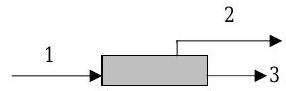
Figure \(\PageIndex{1}\): A device with one current flowing in and two currents flowing out of it.
The electric currents for the device are given below for the current arrows as shown on the diagram.
\[\begin{align*} \text { Wire 1: } & i_{1}(\mathrm{t})=(9 \mathrm{~mA}) \cdot \cos [t /(6 \mathrm{~s})] \\ \text { Wire 2: } & i_{2}(\mathrm{t})=(6 \mathrm{~mA}) \cdot \exp [-t /(6 \mathrm{~s})] \\ \text { Wire 3: } & i_{3}(t)=(9 \mathrm{~mA}) \cdot \{ 1-\exp [-t /(6 \mathrm{~s})] \} \cdot \cos [(t /(6 \mathrm{~s})] \end{align*} \nonumber \]
(a) Develop an equation that describes the time rate of change of net charge in the device. Plot the rate of change versus time for \(t=0\) to \(60 \mathrm{~s}\). Using this equation alone (and the associated plot), discuss what how you expect the net charge of the device to change for \(t=0\) to \(t>>0\).
(b) Develop an equation for the net charge on the device as a function of time and plot your result for 60 seconds. What is the net charge on the device at \(t = 6, 12, 18, 24, 30\), and \(60 \mathrm{~s}\) ? How does this result compare with your predictions from part (a)?
[Note: Any graphs or plots must be complete plots with titles, labels., etc. Hand drawn or computer generated is acceptable.]
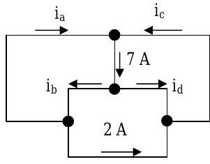
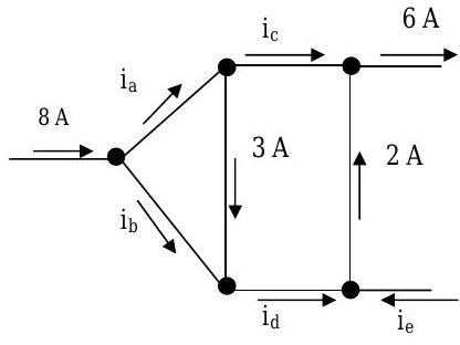
Two different circuits are shown below. Each black dot represents a node and the line connecting two nodes is a branch. The circuits are designed so that there is no accumulation of net charge anywhere in the circuit.
.jpg?revision=1)
.jpg?revision=1)
For each circuit, answer the following questions:
(a) Using only conservation of charge, what is the maximum number of independent equations that you can develop relating the currents in the circuit?
(b) How many unknown currents can you solve for in each problem?
(c) If you have sufficient information, solve for the unknown currents, in amps.
(d) Is there a General Rule here about number of nodes and number of independent current equation? What is it?
Determine the value of the node voltages (measured with respect to ground) and the magnitude and direction of the current flowing in each resistor. Your final answer should include a diagram with labeled with arrows showing current direction and magnitudes and labeled node voltages.
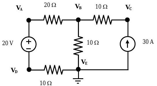
Figure \(\PageIndex{3}\): Circuit diagram with 5 node voltages and 5 branch currents to solve for.
Determine the value of the node voltages (measured with respect to ground) and the magnitude and direction of the current flowing in each resistor. Your final answer should include a diagram with labeled with arrows showing current direction and magnitudes and labeled node voltages.
.jpg?revision=1)
Figure \(\PageIndex{4}\): Circuit diagram with a total of 5 nodes and 7 branches.
For the circuit shown below, solve for the unknown currents and voltages. Make the standard lumped circuit assumptions and assume that all resistances are known and have a value of 2 ohms.
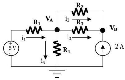
Figure \(\PageIndex{5}\): Circuit digram with 3 node voltages and 4 branch currents to solve for.
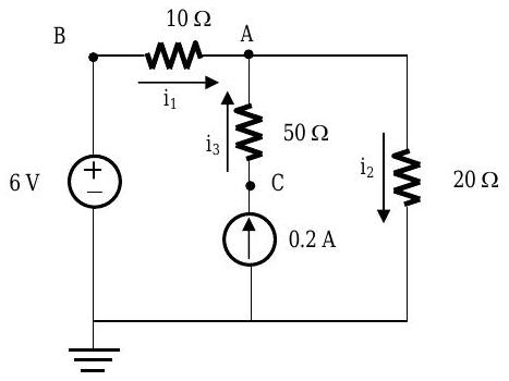
For the circuit shown, determine the currents \(i_{1}\), \(i_{2}\), and \(i_{3}\) and the voltages at \(A, B\), and \(C\) measured with respect to ground.
.jpg?revision=1)
Figure \(\PageIndex{6}\): Circuit with 3 point voltages and 3 branch currents to solve for.
For the circuit shown, determine the unknown currents and node voltages.
.jpg?revision=1)
Figure \(\PageIndex{7}\): Circuit with 3 node voltages and 4 branch currents to solve for.
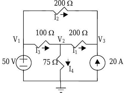
For the circuit shown below, determine the indicated branch currents and node voltages.
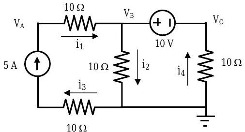
Figure \(\PageIndex{8}\): Circuit with 3 node voltages and 4 branch currents to solve for.
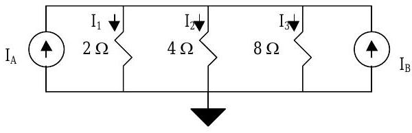
In the circuit shown, the source currents are \(I_{A}=3 \mathrm{~A}\) and \(I_{B}=5 \mathrm{~A} .\) Determine \(I_{1}\), \(I_{2}\), and \(I_{3}\).
.jpg?revision=1)
Figure \(\PageIndex{9}\): Circuit with 3 branch currents to solve for.
Using conservation of charge and Ohm's Law, find the current \(I_{x}\) and voltage \(V_{x}\).
.jpg?revision=1)
Figure \(\PageIndex{10}\): Circuit with one branch current and one node voltage to solve for.
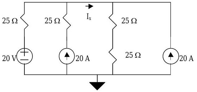
Using conservation of charge and Ohm's Law, find the current \(I_{x}\) and voltage \(V_{x}\).
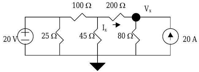
Figure \(\PageIndex{11}\): Circuit with one branch current and one node voltage to solve for.
Using conservation of charge and Ohm's Law, find the current \(I_{x}\) and voltage \(V_{x}\).\
.jpg?revision=1)
Figure \(\PageIndex{12}\): Circuit with one branch current and one node voltage to solve for.
Using conservation of charge and Ohm's Law, find the current \(I_{x}\).
.jpg?revision=1)
Figure \(\PageIndex{13}\): Circuit with one branch current to solve for.
Using conservation of charge and Ohm's Law, find the current \(I_{x}\).
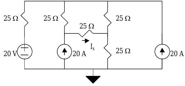
Figure \(\PageIndex{14}\): Circuit with one branch current to solve for.