5.4: Linear Impulse, Linear Momentum, and Impulsive Forces

As we have already demonstrated, it is sometimes necessary to integrate the rate form of the conservation of linear momentum equation over a specified time interval. This gives a relationship between the change of linear momentum within the system and the amount of linear momentum transported into the system. Historically, these types of calculations have been done through the introduction of a quantity known as the linear impulse. Under certain conditions, a system will be subjected to a relatively large force over a very short time interval, such as the contact between two billiard balls or the impact between two cars as they collide. These large, short-duration forces are known as impulsive forces and the interaction is referred to as an impact. In this section we will demonstrate that impact calculations for impulse and impulsive forces follow naturally from our understanding of the basic conservation of linear momentum equation.

5.4.1 Linear Impulse

When a force acts on a system boundary, linear momentum flows across the boundary at a specified rate — the greater the magnitude of the force, the greater the transport rate of linear momentum. If we consider a simple particle with a single force \(\mathbf{F}\) acting on it, we know that the rate of change of the linear momentum of the system is \[\frac{d \mathbf{P}_{\mathrm{sys}}}{d t}=\mathbf{F} \nonumber \]

By definition, the linear impulse of the force \(\mathbf{F}\) is the integral of the force with respect to time: \[\mathbf{Impulse }_{t_{1} \rightarrow t_{2}} = \int\limits_{t_{1}}^{t_{2}} \mathbf{F} \ dt \nonumber \]

As can be seen in Figure \(\PageIndex{1}\), this represents the area under a \(\mathbf{F}\)-\(t\) curve.

Figure \(\PageIndex{1}\): \(\mathbf{F}\)-\(t\) curve.

For the particle, we see that the impulse of force \(\mathbf{F}\) just equals the change in linear momentum of the particle: \[\mathbf{Impulse} \left. \right|_{\mathbf{F}, \ t_{1} \rightarrow t_{2}} = \int\limits_{t_{1}}^{t_{2}} \mathbf{F} \ dt = \int\limits_{t_{1}}^{t_{2}} \left( \frac{d \mathbf{P}_{\mathrm{sys}}}{d t} \right) dt = \mathbf{P}_{\mathrm{sys}, 2}-\mathbf{P}_{\mathrm{sys}, 1} \nonumber \]

For any system, the impulse of a given force equals the amount of linear momentum transferred across the system boundary in the specified time interval. It does not always equal the change in linear momentum of the system. Frequently, it is impossible to directly measure the magnitude of the force as a function of time. In this case, it is common practice to talk about the impulse of the force and, if possible, to determine the impulse by measuring the change in linear momentum of the system.

5.4.2 Impulsive Forces

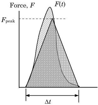
The inability to measure the details of a given force as a function of time is especially true during impacts. An impulsive force is a relatively large force that acts over a very short time period — for instance, when a bowling ball hits a bowling pin. When this occurs, the bowling ball transfers linear momentum to the pin by a short-duration contact force. The same thing would be true of the linear momentum imparted to a homerun pitch as the baseball impacts the slugger's bat for a very short period of time. For a very small interval of time, it is possible to estimate the magnitude of the average impulsive force by assuming that the force is constant over the small time interval: \[\mathbf{F}_{\text {avg }} \Delta t = \int\limits_{t}^{t+\Delta t} \mathbf{F} \ dt = \left. \mathbf{Impulse} \right|_{\mathbf{F}, \ t_{1} \rightarrow t_{2}} \quad \rightarrow \quad \mathbf{F}_{\text {avg}} = \frac{1}{\Delta t} \int\limits_{t}^{t+\Delta t} \mathbf{F} \ dt \nonumber \] As shown in Figure \(\PageIndex{2}\), the average impulsive force equals the constant force that acts over the same time interval and transfers the same amount of linear momentum as the original time-varying force.

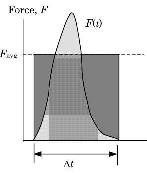
Figure \(\PageIndex{2}\): Impulsive force.

Test Your Understanding — Estimating the peak force during impulse loading

In calculating the average impulsive force above we have assumed that the shape and the area of the \(\mathbf{F}\)-\(t\) curve can best be approximated by a rectangular box of height \(F_{\text {avg}}\) and width \(\Delta t\). There are other possible shapes we could use to approximate the \(\mathbf{F}\)-\(t\) curve. Suppose we approximated the area under the \(\mathbf{F}\)-\(t\) curve using an isosceles triangle of height \(F_{\text {peak}}\) and base \(\Delta t\).

What is the relationship between \(F_{\text {avg}}\) and \(F_{\text {peak}}\) for a impulsive loading situation of duration \(\Delta t\) ? Which value gives a better estimate of the maximum force experienced by the system during the impact and why is it better?

Figure \(\PageIndex{3}\): Impulsive force approximation using isosceles triangle.

Example — Colliding boxcars

Two boxcars are to be coupled together in a railroad switchyard. Boxcar A is moving to the right with a velocity of \(3 \mathrm{~km} / \mathrm{h}\) and is to be coupled to boxcar B, which is initially stationary. Boxcar A has a mass of \(45,000 \mathrm{~kg}\) and boxcar B has a mass of \(25,000 \mathrm{~kg}\).

Determine (a) the final velocity of the coupled cars, and (b) the average impulsive force acting on each car during the coupling if the coupling process takes \(0.3 \ \text{s}\).

Solution

Known: Two boxcars collide and are coupled together.

Find: (a) final velocity of the coupled cars

(b) average impulsive force on cars if coupling process takes \(0.3 \ \text{s}\).

Given:

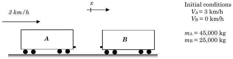
Figure \(\PageIndex{4}\): Initial conditions and relative positions of two boxcars.

Analysis:

Strategy \(\rightarrow\) Since this problem involves two objects colliding with an impact, try looking at conservation of linear momentum.

System \(\rightarrow\) I'm not sure yet, I'll decide this in a minute.

Property to count \(\rightarrow\) Linear momentum in the \(x\)-direction.

Time interval \(\rightarrow\) Finite time since interested in behavior before and after.

Now consider what system to pick. Let's try using a moving closed system that includes only the boxcars.

Figure \(\PageIndex{5}\): Choice of system, before and after the collision.

Notice that if we only consider \(x\)-momentum, there are no forces acting on the system with a component in the \(x\)-direction. So the conservation of linear momentum equation becomes \[\frac{d P_{x, \ \text{sys}}}{dt} = \sum \underbrace{F_{x \ \text {external}}}_{\text {No } x \text{-forces}} + \underbrace{ \sum_{i} \cancel{ \dot{m} V_{x, i} }^{=0} - \sum_{e} \cancel{ \dot{m} V_{x, e} }^{=0} }_{\text {Closed System}} \rightarrow P_{x, \ \text{sys}} = \text {constant} \nonumber \]

Using this result to relate the linear momentum of the system before and after the impact gives the following: \[\begin{gathered} &P_{x, \ 1} = m_{A} V_{A, \ 1} + m_{B} \cancel{V_{B, \ 1}}^{=0} \\ &P_{x, 2} = m_{A} \cancel{ V_{A, \ 2} }^{=V_{2}} +m_{B} \cancel{ V_{B, 2} }^{=V_{2}} \end{gathered} \rightarrow \quad \rightarrow \quad \begin{gathered} P_{x, \ 1} = P_{x, \ 2} \\ m_A V_{A, \ 1} = \left( m_{A}+m_{B} \right) V_{2} \end{gathered} \quad \rightarrow \quad V_{2} = \frac{m_{A}}{\left(m_{A} + m_{B}\right)} V_{A, \ 1} \nonumber \]

Solving for the final velocity we have \(V_{2} = \dfrac{m_{A}}{\left(m_{A}+m_{B}\right)} V_{A, \ 1} = \dfrac{45}{(45+25)}\left(3 \ \dfrac{\mathrm{km}}{\mathrm{h}}\right) = 1.93 \mathrm{~km} / \mathrm{h}\).

And since this is a positive number, the coupled trains will continue to move to the right (positive \(x\)-direction). This is the answer to Part (a).

Now to determine the average impulsive force, we must place a boundary where the force occurs. Consider a closed system that includes only boxcar B. Starting with the conservation of linear momentum for this closed system gives \( \dfrac{d P_{x, \ \text{sys}}}{d t} = F_{\text {coupling}} \).

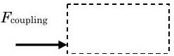
Figure \(\PageIndex{6}\): Closed system consisting of Boxcar B.

But to find the average coupling force on car B, we must integrate this expression over the time interval: \[\int\limits_{t_{1}}^{t_{2}} \left( \frac{d P_{x, \ \text{sys}}}{d t} \right) dt = \int\limits_{t_{1}}^{t_{2}} F_{\text {coupling }} dt \quad \rightarrow \quad P_{x, \ 2} - P_{x, \ 1} = F_{\text {coupling, avg }} \Delta t \nonumber \] Solving for the force we have \[\begin{aligned} F_{\text {coupling, avg}} &= \frac{P_{x, \ 2}-P_{x, \ 1}}{\Delta t} = m_{B} \frac{V_{B, \ 2}-V_{B, \ 1}}{\Delta t} \\[4pt] &=(25,000 \mathrm{~kg}) \left[ \frac{(1.93-0) \ \dfrac{\mathrm{m}}{\mathrm{h}}}{(0.3 \mathrm{~s})} \right] \left( \frac{\mathrm{h}}{3600 \mathrm{~s}} \right) \left( \frac{\mathrm{N} \cdot \mathrm{s}^{2}}{\mathrm{kg} \cdot \mathrm{m}} \right) = 44.7 \times 10^{3} \mathrm{~N} = 44.7 \ \mathrm{kN} \end{aligned} \nonumber \]

Since the value is positive, the direction of the coupling force on car B is as shown in the figure. The coupling force acting on car A is of the same magnitude and opposite direction.

Comment

(1) Consider an alternate system for solving Part (a). This time assume an open system that initially includes car B and finally includes both cars.

Starting with the linear momentum equation: \[ \frac{d P_{x, \ \text{sys}}}{dt} = \underbrace{ \sum \cancel{ F_x }^{=0} }_{\text{No forces in } x \text{-direction} } + \,\,\,\, \dot{m}_i V_{x, \ i} \,\,\,\, - \underbrace{ \cancel{ \dot{m}_e V_e }^{=0} }_{\text{No flow out of system}} \quad\quad \rightarrow \quad\quad \frac{ d P_{x, \ \text{sys}} }{dt} = \underbrace{ \dot{m}_i V_{x, \ i} }_{\begin{array}{c} x \text{-momentum carried} \\ \text{in with boxcar A} \end{array} } \nonumber \]

To find the velocity (or linear momentum) of the system after the coupling we must integrate this equation over the time interval: \[ \int\limits_{t_1}^{t_2} \left( \frac{d P_{x, \ \text{sys}}}{dt} \right) dt = \underbrace{ \int\limits_{t_1}^{t_2} \left( \dot{m}_i V_i \right) dt }_{\begin{array}{c} = \text{ all of the momentum} \\ \text{carried into the system} \\ \text{by boxcar A} \end{array}} \quad \rightarrow \quad \underbrace{ P_{x, \ 2} }_{\begin{array}{c} \text{Includes} \\ \text{both cars} \end{array}} - \underbrace{ P_{x, \ 1} }_{\begin{array}{c} \text{Only} \\ \text{car B} \end{array}} = m_A V_A \quad\quad \rightarrow \quad\quad \left( m_A + m_B \right) V_2 = m_A V_A \nonumber \]

The solution continues on from this point as above. Notice how starting with a different system, even an open system, we can recover the same equation using consistent assumptions. This illustrates that is often possible to solve the same problem using several different systems.

(2) Select an open system that has mass flowing in and out during the impact and solve for the final velocity of the coupled cars. [Hint: This system would have no linear momentum in either the initial or final states.]

(3) How long would it take the coupled cars to come to a complete stop if the brakes on car B were locked at the time of impact and the coefficient of kinetic friction between the wheels and the rail is \(0.10\)? What would the velocity of the coupled cars be immediately after the impact? Would it be reasonable to neglect the friction force during the impact? [Answer: \(1.53\) seconds].