
5.5: Linear Momentum Revisited
- Page ID
- 83082
This section considers additional aspects of calculating linear momentum. The first subsection considers the use of relative velocities and the second subsection addresses the use of cylindrical coordinates to describe curvilinear plane motion.
Using Relative Velocities
The following example illustrates how conservation of linear momentum can be used to solve for the motion of a rocket that is accelerating. This example makes use of relative velocities.
A small rocket fully loaded with fuel and oxidizer has a mass of \(500 \ \mathrm{Mg}\), and \(80 \%\) of the total mass is fuel and oxidizer. The rocket is pointed vertically up and is placed on a launching pad on the surface of Earth. After ignition, the mass flow rate of the exhaust from the rocket engine is \(2300 \mathrm{~kg} / \mathrm{s}\) with an exit velocity of \(2100 \mathrm{~m} / \mathrm{s}\) relative to the rocket. Neglecting pressure forces and fluid drag, determine (a) how long after ignition does burnout occur (i.e. the rocket runs out of fuel and oxidizer)? (b) how long after ignition does liftoff occur? and (c) what is the velocity of the rocket at burnout?
Solution
Known: A small rocket takes off from the surface of the earth.
Find: (a) time after ignition until burnout; (b) time after ignition until liftoff; (c) velocity of the rocket at burnout.
Given:
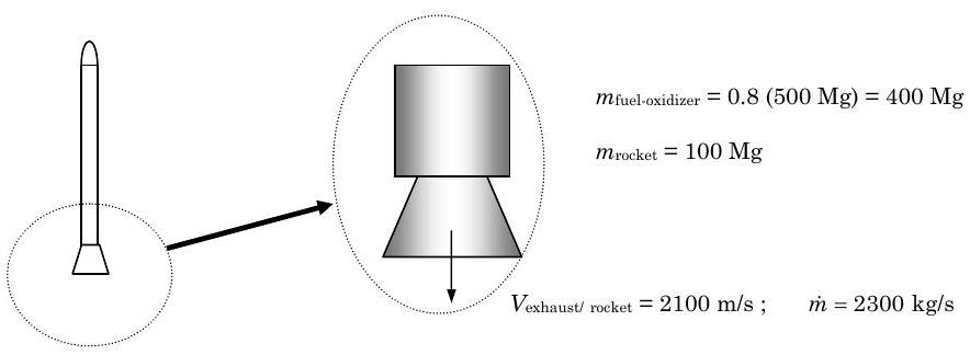
Figure \(\PageIndex{1}\): Given information.
Analysis:
Strategy \(\rightarrow\) Since we are concerned about velocity of an accelerating object and about the time needed to run out of the mass of fuel and oxidizer, let's try using mass and linear momentum.
System \(\rightarrow\) Take an open, non-deforming system which includes the rocket with mass crossing the boundary at the exhaust.
Property to count \(\rightarrow\) As stated above, try mass and linear momentum.
Time interval \(\rightarrow\) Start with rate form and then see what's needed.
.png?revision=1)
Figure \(\PageIndex{2}\): Choice of system and direction of mass flow across boundary.
For the system above, the mass flows out of the bottom of the rocket as indicated by the arrow. To solve part (a), write the conservation of mass for the system; then by integrating with time, we have: \[\begin{align*} \frac{d m_{\text{sys}}}{dt} = -\dot{m}_{e} \quad & \rightarrow \quad \int\limits_{t_{1}}^{t_{2}} \left(\frac{d m_{\text{sys}}}{dt}\right) dt = \int\limits_{t_{1}}^{t_{2}} \left(-\dot{m}_{e}\right) dt \quad \rightarrow \quad m - m_{o} = -\dot{m}_{e} t \\ m = m_{o} - \dot{m}_{e} t \quad & \rightarrow \quad m=(500,000 \mathrm{~kg}) - \left( 2300 \ \frac{\mathrm{kg}}{\mathrm{s}}\right) t \end{align*} \nonumber \]
Notice that the mass flow rate is calculated with respect to the rocket exhaust. At burnout, the mass of the system equals just the mass of the empty rocket: \[t_{\text {burnout}} = \frac{(500,000 \mathrm{~kg} - 100,000 \mathrm{~kg})}{\left(2300 \ \dfrac{\mathrm{kg}}{\mathrm{s}}\right)} = 173.9 \text { seconds } \nonumber \]
Now to solve for the liftoff time, we need to apply the conservation of linear momentum: \[ \begin{align*} \boxed{ \uparrow + } \quad\quad\quad\quad\quad\quad\quad\quad \frac{d P_{y, \ \text{sys}}}{dt} &= -mg - \dot{m}_e V_{y, \ e} \\[4pt] \frac{d \left( m V_G \right)}{dt} &= -mg - \dot{m}_e \underbrace{ \left( V_G - V_{\text{exhaust / rocket}} \right) }_{\begin{array}{c} \text{Absolute velocity of the exhaust} \\ \text{with respect to the ground} \end{array}} \\ m \frac{d V_G}{dt} + V_G \underbrace{ \cancel{ \frac{dm}{dt} }^{= - \dot{m}_e} }_{\begin{array}{c} \text{Using conservation} \\ \text{of mass results} \end{array}} &= -mg - \dot{m}_e \left( V_G - V_{\text{exhaust / rocket}} \right) \\ m \frac{d V_G}{dt} + V_G \left( - \dot{m}_e \right) &= -mg - \dot{m}_e \left( V_G - V_{\text{exhaust / rocket}} \right) \\ m \frac{d V_G}{dt} &= -mg - \dot{m}_e \left( V_G - V_{\text{exhaust / rocket}} \right) + \dot{m}_e V_G \\[4pt] m \frac{d V_G}{dt} &= -mg - \cancel{ \dot{m}_e V_G } + \dot{m}_e V_{\text{exhaust / rocket}} + \cancel{ \dot{m}_e V_G } \\[8pt] m \frac{d V_G}{dt} &= -mg + \dot{m}_e V_{\text{exhaust / rocket}} \end{align*} \nonumber \]
Carefully study the steps above. Note that you must be careful to use the absolute velocity of the exhaust leaving the exhaust. Also note that we make use of the conservation of mass equation in simplifying the conservation of linear momentum.
To solve for part (b), the liftoff time, we can use the equation above. At liftoff the acceleration of the system is zero, as the thrust just balances the weight of gravity: \[m \cancel{ \frac{d V_G}{d t} }^{=0} = -mg + \dot{m}_{e} V_{\text {exhaust / rocket }} \quad \rightarrow \quad \begin{gathered} mg = \dot{m}_{e} V_{\text {exhaust / rocket}} \\ \left(m_{o}-\dot{m}_{e} t \right) g = \dot{m}_{e} V_{\text {exhaust / rocket}} \\ m_{o} g = \dot{m}_{e} \left(gt + V_{\text {exhaust / rocket}}\right) \end{gathered} \quad \rightarrow \quad t_{\text {liftoff}} = \frac{m_{o}}{\dot{m}_{e}} - \frac{V_{\text {exhaust / rocket}}}{g} \nonumber \]
Then solving for the liftoff time: \[t_{\text {liftoff}} = \frac{m_{o}}{\dot{m}_{e}} - \frac{V_{\text {exhaust / rocket}}}{g} = \left(\frac{500,000 \mathrm{~kg}}{2300 \mathrm{~kg} / \mathrm{s}}\right) - \left(\frac{2100 \mathrm{~m} / \mathrm{s}}{9.81 \mathrm{~m} / \mathrm{s}^{2}} \right) = 3.32 \mathrm{~seconds} \nonumber \]
Finally to solve for the velocity at burnout, we must calculate the velocity of the rocket as a function of time. We do this by integrating the acceleration equation for the rocket. First rearranging the conservation of linear momentum result, we have an expression for the acceleration of the rocket: \[\frac{d V_{G}}{d t} = -g + \frac{\dot{m}_{e}}{m} V_{\text {exhaust / rocket }} \nonumber \]
Integrating this with time from the point of liftoff gives the following: \[ \begin{align*} \int\limits_{t_{\text{liftoff}}}^{t} \left( \frac{d V_G}{dt} \right) dt &= \int\limits_{t_{\text{liftoff}}}^{t} \left[ -g + \frac{\dot{m}_e V_{\text{exhaust / rocket}}}{\left( m_o - \dot{m}_e t \right)} \right] dt \\[4pt] \left. V_G - V_G \right|_{t_{\text{liftoff}}} &= \int\limits_{t_{\text{liftoff}}}^{t} \left[ -g \right] dt + \int\limits_{t_{\text{liftoff}}}^{t} \left[ \frac{\dot{m}_e V_{\text{exhaust / rocket}}}{\left( m_o - \dot{m}_e t \right)} \right] dt \\[4pt] V_G - \cancel{ \left. V_G \right|_{t_{\text{liftoff}}} }^{=0} &= -g \left( t - t_{\text{liftoff}} \right) + \dot{m}_e V_{\text{exhaust / rocket}} \left[ \frac{1}{\dot{m}_e} \int\limits_{t_{\text{liftoff}}}^{t} \frac{\dot{m}_e \ dt}{\left( m_o - \dot{m}_e t \right) } \right] \\[4pt] V_G &= -g \left( t - t_{\text{liftoff}} \right) + \dot{m}_e V_{\text{exhaust / rocket}} \left[ - \frac{1}{\dot{m}_e} \ \ln \left( \frac{m_o - \dot{m}_e t}{m_o - \dot{m}_e t_{\text{liftoff}}} \right) \right] \\[10pt] V_G &= -g \left( t - t_{\text{liftoff}} \right) - V_{\text{exhaust / rocket}} \left[ \ln \left( \frac{m_o - \dot{m}_e t}{m_o - \dot{m}_e t_{\text{liftoff}}} \right) \right] \end{align*} \nonumber \]
Note that this equation is only valid for \(t_{\text {liftoff}} \leq t \leq t_{\text {burnout}}\). Solving for the velocity at burnout gives \[\begin{aligned} V_{G} &= -g \left(t_{\text {burnout}} - t_{\text {liftoff}}\right) - V_{\text {exhaust / rocket}} \left[\ln \left(\frac{m_{o}-\dot{m}_{e} t_{\text {burnout}}}{m_{o}-\dot{m}_{e} t_{\text {liftoff}}}\right)\right] \\[4pt] &= -\left(9.81 \ \frac{\mathrm{kg}}{\mathrm{s}}\right)(173.9-3.32) \mathrm{s}-\left(2100 \ \frac{\mathrm{m}}{\mathrm{s}}\right) \left[\ln \frac{(100 \ \mathrm{Mg})}{\left(500 \ \mathrm{Mg}-2.3 \ \dfrac{\mathrm{Mg}}{\mathrm{s}}(3.32 \mathrm{~s})\right)}\right] \\[4pt] &=\left(-1673 \ \frac{\mathrm{m}}{\mathrm{s}}\right) - \left(-3348 \ \frac{\mathrm{m}}{\mathrm{s}}\right) \\[4pt] &= 1675 \mathrm{~m} / \mathrm{s} \end{aligned} \nonumber \]
Comments
How far above the earth would the rocket be at burnout? How could you calculate this? Do you think our model is accurate all the way to burnout? What possible problems would you see?
If the diameter of the rocket nozzle exhaust is \(5 \mathrm{~m}\) and the exhaust pressure is \(10 \ \mathrm{kPa}\), determine the net pressure force on the system. Assume atmospheric pressure is \(100 \ \mathrm{kPa}\). Was neglecting the pressure force reasonable?
Motion with Cylindrical Coordinates
The following application shows how cylindrical coordinates can be used to describe plane curvilinear motion.
Sometimes it is advantageous to describe the motion of a point in a plane in terms of the distance \(r\) from the origin and the angle \(\theta\) measured from the positive \(x\)-axis, i.e. cylindrical coordinates. Using the definitions of velocity and acceleration as first and second derivatives of position with respect to time and the trigonometric relations between \(x, y, r,\) and \(\theta\) the following relationships can be developed:
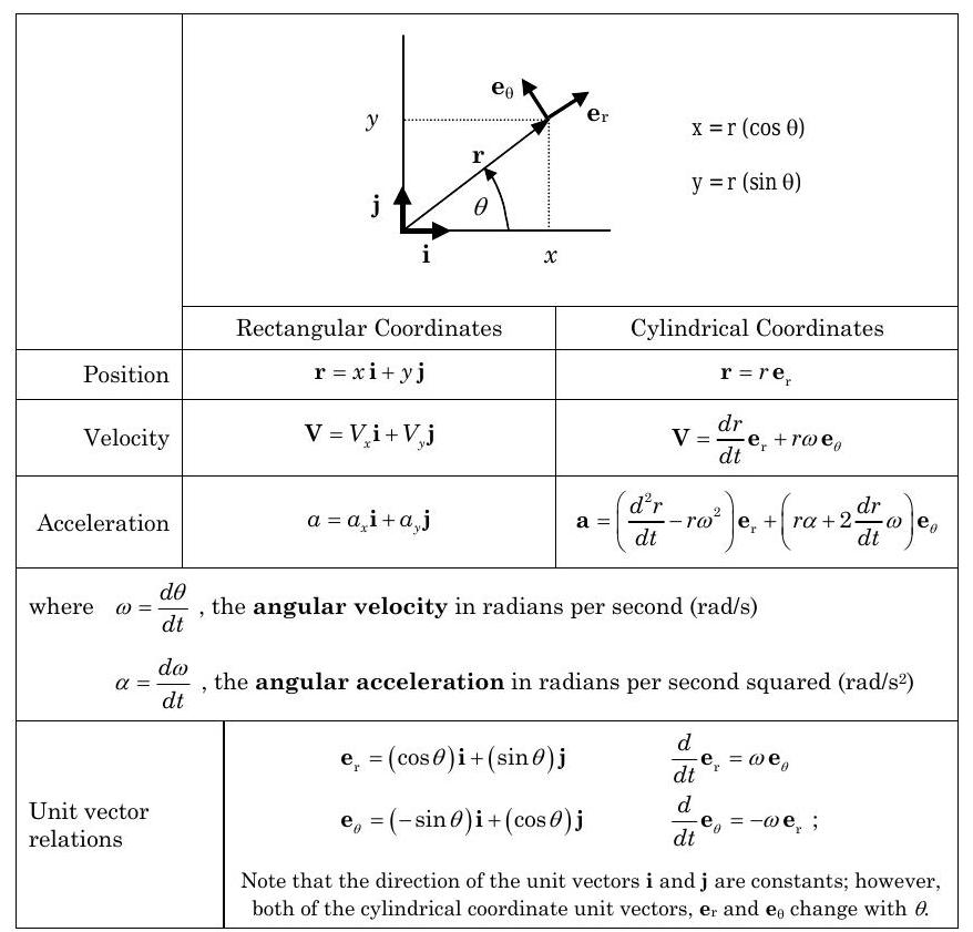
Figure \(\PageIndex{3}\): Table of unit vector and position, velocity, and acceleration equation relationships between rectangular and cylindrical coordinates.
(a) Starting with the position vector \(\mathbf{r}\), show that \(\mathbf{e}_{\mathrm{r}}=(\cos \theta) \mathbf{i}+(\sin \theta) \mathbf{j}\).
(b) Now differentiate \(\mathbf{e}_{\mathbf{r}}\) with respect to time and prove to yourself that \(\dfrac{d}{d t} \mathbf{e}_{\mathbf{r}}=\omega \mathbf{e}_{\theta}\).
(c) How do the relations for \(\mathbf{r}, \mathbf{V}\), and \(\mathbf{a}\) in cylindrical coordinates simplify if \(r=R\), a constant?
(d) How do the relations for \(\mathbf{r}, \mathbf{V}\), and \(\mathbf{a}\) in cylindrical coordinates simplify if \(\omega=\) constant?
A circular disk of radius \(R\) and thickness \(t\) is made of a material with density \(\rho\). Determine the linear momentum for the disk under the following conditions:
(a) The disk is rotating with a rotational velocity \(\omega\) about its centroidal axis, \(G\). Even though this disk appears to touch the ground, it is slipping and is not rolling.
(b) The disk is sliding to the right without rotating, i.e. \(\omega=0\). The disk is translating with velocity \(\mathbf{V}\).
.png?revision=1)
Figure \(\PageIndex{4}\): Given information about disk.
Solution:
Known: A circular disk moves with specified motion.
Find: (a) Linear momentum when the disk is rotating about its centroidal axis.
(b) Linear momentum when the disk is translating with velocity \(\mathbf{V}\).
Given: See figure above.
Analysis: Strategy \(\rightarrow\) Use the definition of linear momentum.
(a) The velocity of the rotating disk measured with respect to the center of mass \(G\) is \(\mathbf{V} = r \omega \mathbf{e}_{\theta} = r \omega \left( -(\sin \theta) \mathbf{i}+(\cos \theta) \mathbf{j} \right)\). Using the definition for linear momentum of a system we have \[\begin{aligned} \mathbf{P}_{\mathrm{sys}} &= \int\limits_{V\kern-0.5em\raise0.3ex-_{\text{sys}}} (\mathbf{V} \rho) d V\kern-1.0em\raise0.3ex- = \int\limits_{0}^{2 \pi} \int\limits_{0}^{R} \underbrace{ \left(r \omega \mathbf{e}_{\theta} \right) }_{\mathbf{V}} \rho \underbrace{ (r \ d \theta \ dr) }_{d V\kern-0.5em\raise0.3ex-} \\ &= (\rho \omega) \int\limits_{0}^{2 \pi} \underbrace{ ((\sin \theta) \mathbf{i} - (\cos \theta) \mathbf{j}) }_{\mathbf{e}_{\theta}} \left( \int\limits_{0}^{R} r^{2} \ dr \right) d \theta = (\rho \omega) \int\limits_{0}^{2 \pi} \underbrace{ ((\sin \theta) \mathbf{i} - (\cos \theta) \mathbf{j}) }_{\mathbf{e}_{\theta}} \left( \frac{R^{3}}{3}\right) d \theta \\ &= \left( \frac{\rho \omega R^{3}}{3} \right) \int\limits_{0}^{2 \pi} \left( (\sin \theta) \mathbf{i} - (\cos \theta) \mathbf{j} \right) \ d \theta \\ &=\left( \frac{\rho \omega R^{3}}{3} \right) \left[ \mathbf{i} \int\limits_{0}^{2 \pi}(\sin \theta) \ d \theta - \mathbf{j} \int_{0}^{2 \pi}(\cos \theta) \ d \theta \right] = \left( \frac{\rho \omega R^{3}}{3} \right)(0)=0 \end{aligned} \nonumber \]
Thus, as you might have guessed the linear momentum of a disk rotating about its centroidal axis is identically zero. In general, the linear momentum of a system rotating about a fixed axis is always zero if (1) the axis of rotation passes through the center of mass, i.e. its centroidal axis, and (2) the system has a plane of symmetry that is perpendicular to the axis of rotation. If either of these two conditions is violated, the linear momentum will not be zero.
Note that this integration could have been simplified greatly if we had used the integral for velocity of the center of mass, Eq. \((5.1.16)\). The center of mass \(G\) of the disk is on the axis of rotation and the axis of rotation is not translating; thus, \[\mathbf{P}_{\mathrm{sys}} = \int\limits_{V\kern-0.5em\raise0.3ex-_{\text{sys}}}(\mathbf{V} \rho) d V\kern-1.0em\raise0.3ex- = m_{s y s} \cancel{ V_{G} }^{=0} =0 \nonumber \] and the linear momentum of the system is zero. This is much easier than doing the full integration!
(b) Starting with the definition of linear momentum and the fact that the disk is translating with velocity \(\mathbf{V}\), we have \[\begin{aligned} \mathbf{P}_{\mathrm{sys}} &= \int\limits_{V\kern-0.5em\raise0.3ex-_{\text {sys}}}(\mathbf{V} \rho) d V\kern-1.0em\raise0.3ex- = \int\limits_{0}^{2 \pi} \int\limits_{0}^{R}(\mathbf{V} \rho) \underbrace{ (rt \ d \theta \ d r)}_{d V\kern-0.5em\raise0.3ex-} = (\mathbf{V} \rho t) \int\limits_{0}^{2 \pi} \int\limits_{0}^{R} r \ dr \ d \theta \\ &=(\mathbf{V} \rho t) \int\limits_{0}^{2 \pi} \left(\int\limits_{0}^{R} r \ dr \right) d \theta = (\mathbf{V} \rho t) \int\limits_{0}^{2 \pi} \left(\frac{R^{2}}{2}\right) d \theta \\ &= (\mathbf{V} \rho t) \left( \frac{R^{2}}{2}\right) \int\limits_{0}^{2 \pi} d \theta =(\mathbf{V} \rho t) \left(\frac{R^{2}}{2}\right)(2 \pi) \\ &= \underbrace{ \left( \rho \left(\pi R^{2} t\right)\right) }_{\rho V\kern-0.5em\raise0.3ex- _{\text{sys}}} \mathbf{V} = m_{sys} \mathbf{V} \end{aligned} \nonumber \]
Thus the linear momentum is just the product of the translational velocity and the system mass. Again, this calculation can be greatly simplified using the equation for the velocity of the center of mass: \[\mathbf{P}_{\mathrm{sys}}=\int_{V\kern-0.5em\raise0.3ex-_{\text{sys}}} (\mathbf{V} \rho) d V\kern-1.0em\raise0.3ex- = m_{s y s} \cancel{ \mathbf{V}_{G} }^{=\mathrm{V}} = m_{sys} \mathbf{V} \nonumber \]