
14.4.1: Circles
- Page ID
- 67364
\( \newcommand{\vecs}[1]{\overset { \scriptstyle \rightharpoonup} {\mathbf{#1}} } \)
\( \newcommand{\vecd}[1]{\overset{-\!-\!\rightharpoonup}{\vphantom{a}\smash {#1}}} \)
\( \newcommand{\dsum}{\displaystyle\sum\limits} \)
\( \newcommand{\dint}{\displaystyle\int\limits} \)
\( \newcommand{\dlim}{\displaystyle\lim\limits} \)
\( \newcommand{\id}{\mathrm{id}}\) \( \newcommand{\Span}{\mathrm{span}}\)
( \newcommand{\kernel}{\mathrm{null}\,}\) \( \newcommand{\range}{\mathrm{range}\,}\)
\( \newcommand{\RealPart}{\mathrm{Re}}\) \( \newcommand{\ImaginaryPart}{\mathrm{Im}}\)
\( \newcommand{\Argument}{\mathrm{Arg}}\) \( \newcommand{\norm}[1]{\| #1 \|}\)
\( \newcommand{\inner}[2]{\langle #1, #2 \rangle}\)
\( \newcommand{\Span}{\mathrm{span}}\)
\( \newcommand{\id}{\mathrm{id}}\)
\( \newcommand{\Span}{\mathrm{span}}\)
\( \newcommand{\kernel}{\mathrm{null}\,}\)
\( \newcommand{\range}{\mathrm{range}\,}\)
\( \newcommand{\RealPart}{\mathrm{Re}}\)
\( \newcommand{\ImaginaryPart}{\mathrm{Im}}\)
\( \newcommand{\Argument}{\mathrm{Arg}}\)
\( \newcommand{\norm}[1]{\| #1 \|}\)
\( \newcommand{\inner}[2]{\langle #1, #2 \rangle}\)
\( \newcommand{\Span}{\mathrm{span}}\) \( \newcommand{\AA}{\unicode[.8,0]{x212B}}\)
\( \newcommand{\vectorA}[1]{\vec{#1}} % arrow\)
\( \newcommand{\vectorAt}[1]{\vec{\text{#1}}} % arrow\)
\( \newcommand{\vectorB}[1]{\overset { \scriptstyle \rightharpoonup} {\mathbf{#1}} } \)
\( \newcommand{\vectorC}[1]{\textbf{#1}} \)
\( \newcommand{\vectorD}[1]{\overrightarrow{#1}} \)
\( \newcommand{\vectorDt}[1]{\overrightarrow{\text{#1}}} \)
\( \newcommand{\vectE}[1]{\overset{-\!-\!\rightharpoonup}{\vphantom{a}\smash{\mathbf {#1}}}} \)
\( \newcommand{\vecs}[1]{\overset { \scriptstyle \rightharpoonup} {\mathbf{#1}} } \)
\(\newcommand{\longvect}{\overrightarrow}\)
\( \newcommand{\vecd}[1]{\overset{-\!-\!\rightharpoonup}{\vphantom{a}\smash {#1}}} \)
\(\newcommand{\avec}{\mathbf a}\) \(\newcommand{\bvec}{\mathbf b}\) \(\newcommand{\cvec}{\mathbf c}\) \(\newcommand{\dvec}{\mathbf d}\) \(\newcommand{\dtil}{\widetilde{\mathbf d}}\) \(\newcommand{\evec}{\mathbf e}\) \(\newcommand{\fvec}{\mathbf f}\) \(\newcommand{\nvec}{\mathbf n}\) \(\newcommand{\pvec}{\mathbf p}\) \(\newcommand{\qvec}{\mathbf q}\) \(\newcommand{\svec}{\mathbf s}\) \(\newcommand{\tvec}{\mathbf t}\) \(\newcommand{\uvec}{\mathbf u}\) \(\newcommand{\vvec}{\mathbf v}\) \(\newcommand{\wvec}{\mathbf w}\) \(\newcommand{\xvec}{\mathbf x}\) \(\newcommand{\yvec}{\mathbf y}\) \(\newcommand{\zvec}{\mathbf z}\) \(\newcommand{\rvec}{\mathbf r}\) \(\newcommand{\mvec}{\mathbf m}\) \(\newcommand{\zerovec}{\mathbf 0}\) \(\newcommand{\onevec}{\mathbf 1}\) \(\newcommand{\real}{\mathbb R}\) \(\newcommand{\twovec}[2]{\left[\begin{array}{r}#1 \\ #2 \end{array}\right]}\) \(\newcommand{\ctwovec}[2]{\left[\begin{array}{c}#1 \\ #2 \end{array}\right]}\) \(\newcommand{\threevec}[3]{\left[\begin{array}{r}#1 \\ #2 \\ #3 \end{array}\right]}\) \(\newcommand{\cthreevec}[3]{\left[\begin{array}{c}#1 \\ #2 \\ #3 \end{array}\right]}\) \(\newcommand{\fourvec}[4]{\left[\begin{array}{r}#1 \\ #2 \\ #3 \\ #4 \end{array}\right]}\) \(\newcommand{\cfourvec}[4]{\left[\begin{array}{c}#1 \\ #2 \\ #3 \\ #4 \end{array}\right]}\) \(\newcommand{\fivevec}[5]{\left[\begin{array}{r}#1 \\ #2 \\ #3 \\ #4 \\ #5 \\ \end{array}\right]}\) \(\newcommand{\cfivevec}[5]{\left[\begin{array}{c}#1 \\ #2 \\ #3 \\ #4 \\ #5 \\ \end{array}\right]}\) \(\newcommand{\mattwo}[4]{\left[\begin{array}{rr}#1 \amp #2 \\ #3 \amp #4 \\ \end{array}\right]}\) \(\newcommand{\laspan}[1]{\text{Span}\{#1\}}\) \(\newcommand{\bcal}{\cal B}\) \(\newcommand{\ccal}{\cal C}\) \(\newcommand{\scal}{\cal S}\) \(\newcommand{\wcal}{\cal W}\) \(\newcommand{\ecal}{\cal E}\) \(\newcommand{\coords}[2]{\left\{#1\right\}_{#2}}\) \(\newcommand{\gray}[1]{\color{gray}{#1}}\) \(\newcommand{\lgray}[1]{\color{lightgray}{#1}}\) \(\newcommand{\rank}{\operatorname{rank}}\) \(\newcommand{\row}{\text{Row}}\) \(\newcommand{\col}{\text{Col}}\) \(\renewcommand{\row}{\text{Row}}\) \(\newcommand{\nul}{\text{Nul}}\) \(\newcommand{\var}{\text{Var}}\) \(\newcommand{\corr}{\text{corr}}\) \(\newcommand{\len}[1]{\left|#1\right|}\) \(\newcommand{\bbar}{\overline{\bvec}}\) \(\newcommand{\bhat}{\widehat{\bvec}}\) \(\newcommand{\bperp}{\bvec^\perp}\) \(\newcommand{\xhat}{\widehat{\xvec}}\) \(\newcommand{\vhat}{\widehat{\vvec}}\) \(\newcommand{\uhat}{\widehat{\uvec}}\) \(\newcommand{\what}{\widehat{\wvec}}\) \(\newcommand{\Sighat}{\widehat{\Sigma}}\) \(\newcommand{\lt}{<}\) \(\newcommand{\gt}{>}\) \(\newcommand{\amp}{&}\) \(\definecolor{fillinmathshade}{gray}{0.9}\)A circle
A circle can be determined by fixing a point at the center and a positive number, the radius.
Definition \(\PageIndex{1}\): Circles
A circle with center \((h,k)\) and radius \(r>0\) is the set of all points \((x, y)\) in the plane whose distance to \((h,k)\) is \(r\).
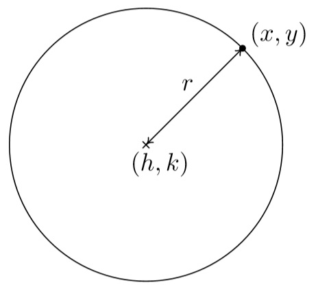
From the picture, we see that a point \((x,y)\) is on the circle if and only if its distance to \((h,k)\) is \(r\). We express this relationship algebraically using the Distance Formula (Equation \ref{distanceformula}), as
\[r = \sqrt{(x - h)^2 + (y-k)^2} \label{distanceformula}\]
By squaring both sides of this equation, we get an equivalent equation (since \(r > 0\)) which gives us the standard equation of a circle.
The Equation of a Circle
Note \(\PageIndex{1}\): The Standard Equation of a Circle
The equation of a circle with center \((h,k)\) and radius \(r >0\) is
\[(x-h)^2 + (y-k)^2 = r^2. \label{standardcircle}\]
or
$$\dfrac{(x-h)^2}{r^2} + \dfrac{(y-k)}{r^2} = 1$$
The second form of the equation is for comparison to hyperbolas and ellipses coming in later sections.
Example \(\PageIndex{1}\): The Standard Equation
Write the standard equation of the circle with center (−2,3) and radius 5.
Solution.
Here, \((h,k) = (-2,3)\) and \(r = 5\), so we get
\[\begin{array}{rcl} (x-(-2))^2+(y-3)^2 &= &(5)^2 \\ (x+2)^2+(y-3)^2 & = & 25 \end{array} \nonumber\]
Example \(\PageIndex{2}\):
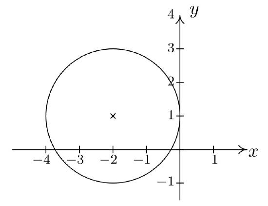
Graph \((x+2)^2+(y-1)^2 = 4\). Find the center and radius.
Solution
From the standard form of a circle, Equation \ref{standardcircle}, we have that \(x + 2\) is \(x-h\), so \(h = -2\) and \(y - 1\) is \(y - k\) so \(k = 1\). This tells us that our center is \((-2,1)\). Furthermore, \(r^2 = 4\), so \(r = 2\). Thus we have a circle centered at \((-2,1)\) with a radius of \(2\). Graphing gives us
If we were to expand the equation in the previous example and gather up like terms, instead of the easily recognizable \((x+2)^2 + (y-1)^2 = 4\), we'd be contending with \(x^2 + 4x + y^2 - 2y + 1 = 0.\) If we're given such an equation, we can complete the square in each of the variables to see if it fits the form given in Equation \ref{standardcircle} by following the steps given below.
To Write the Equation of a Circle in Standard Form
- Group the same variables together on one side of the equation and position the constant on the other side.
- Complete the square on both variables as needed.
- Divide both sides by the coefficient of the squares. (For circles, they will be the same.)
Example \(\PageIndex{3}\):
Complete the square to find the center and radius of \(3x^2 - 6x + 3y^2 + 4y -4 = 0\).
Solution
\[ \begin{array}{rclr} 3x^2 - 6x + 3y^2 + 4y -4 & = & 0 & \\ 3x^2 - 6x + 3y^2 + 4y & = & 4 & \mbox{add \(4\) to both sides} \\ 3\left(x^2 - 2x \right) + 3\left(y^2 + \dfrac{4}{3} y\right) & = & 4 & \mbox{factor out leading coefficients} \\ 3\left(x^2 - 2x + \underline{1} \right) + 3\left(y^2 + \dfrac{4}{3} y + \underline{\underline{\dfrac{4}{9}}} \right) & = & 4 + 3\underline{(1)} + 3\underline{\underline{\left(\dfrac{4}{9}\right)}} & \mbox{complete the square in \(x\), \(y\)} \\ 3(x - 1)^2 + 3\left(y + \dfrac{2}{3}\right)^2 & = & \dfrac{25}{3} & \mbox{factor} \\ (x - 1)^2 + \left(y + \dfrac{2}{3}\right)^2 & = & \dfrac{25}{9} & \mbox{divide both sides by \(3\)}\end{array} \]
From Equation \ref{standardcircle}, we identify \(x - 1\) as \(x - h\), so \(h = 1\), and \(y + \frac{2}{3}\) as \(y - k\), so \(k = - \frac{2}{3}\). Hence, the center is \((h,k) = \left(1, -\frac{2}{3}\right)\). Furthermore, we see that \(r^2 = \frac{25}{9}\) so the radius is \(r = \frac{5}{3}\).
It is possible to obtain equations like \((x-3)^2 + (y+1)^2 = 0\) or \((x-3)^2 + (y+1)^2 = -1\), neither of which describes a circle. The reader is encouraged to think about what, if any, points lie on the graphs of these two equations.
Example \(\PageIndex{4}\):
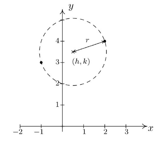
Write the standard equation of the circle which has \((-1,3)\) and \((2,4)\) as the endpoints of a diameter.
Solution
We recall that a diameter of a circle is a line segment containing the center and two points on the circle. Plotting the given data yields
Since the given points are endpoints of a diameter, we know their midpoint \((h, k)\) is the center of the circle. This is easily solved as
\[ \begin{array}{rcl} (h,k) & = & \left( \dfrac{x_{\mbox{1}} + x_{\mbox{2}}}{2}, \dfrac{y_{\mbox{1}} + y_{\mbox{2}}}{2} \right) \\ & = & \left( \dfrac{-1+2}{2}, \dfrac{3+4}{2} \right) \\ & = & \left( \dfrac{1}{2}, \dfrac{7}{2} \right) \end{array} \]
The diameter of the circle is the distance between the given points, so we know that half of the distance is the radius. Thus,
\[ \begin{array}{rcl} r & = & \dfrac{1}{2} \sqrt{\left(x_{\mbox{2}} - x_{\mbox{1}}\right)^2+\left(y_{\mbox{2}}-y_{\mbox{1}}\right)^2} \\ & = & \dfrac{1}{2} \sqrt{(2-(-1))^2+(4-3)^2} \\ & = & \dfrac{1}{2} \sqrt{3^2+1^2} \\ & = &\dfrac{\sqrt{10}}{2} \end{array} \]
Finally, since \(\left( \dfrac{\sqrt{10}}{2} \right)^2 = \dfrac{10}{4}\), our answer becomes \(\left(x - \dfrac{1}{2} \right)^2 + \left(y - \dfrac{7}{2} \right)^2 =\dfrac{10}{4}\)
The Unit Circle
We close this section with an important circle in mathematics1: the Unit Circle.
Definition \(\PageIndex{2}\): Unit Circle
The Unit Circle is the circle centered at \((0,0)\) with a radius of \(1\). The standard equation of the Unit Circle is \(x^2 + y^2 = 1.\)
Example \(\PageIndex{5}\):
Find the points on the unit circle with \(y\)-coordinate \(\dfrac{\sqrt{3}}{2}\).
Solution
We replace \(y\) with \(\dfrac{\sqrt{3}}{2}\) in the equation \(x^2 + y^2 = 1\) to get
\[ \begin{array}{rcl} x^2 + y^2 & = & 1 \\ x^2 + \left(\dfrac{\sqrt{3}}{2}\right)^2 & = & 1 \\ \dfrac{3}{4} + x^2 & = & 1 \\ x^2 & = & \dfrac{1}{4} \\ x & = & \pm \sqrt{\dfrac{1}{4}} \\ x & = & \pm \dfrac{1}{2} \end{array} \]
Our final answers are \(\left(\dfrac{1}{2}, \dfrac{\sqrt{3}}{2} \right)\) and \(\left(-\dfrac{1}{2}, \dfrac{\sqrt{3}}{2} \right)\).
Contributors and Attributions
1The unit circle is used in trigonometry to define and evaluate trigonometric functions like sine and cosine.